
Combinatorics in Probability — Intuitively and Exhaustively Explained
Part 1 of an Introduction to Probability

Probability is a fundamental topic in science, technology, and understanding in general. To a large extent, the modern era is a direct result of humans unlocking the ability to understand and reason with uncertainty. Considering its importance, it seems like something worth learning about.
I set off to describe probability just like any other topic, but found I couldn’t be properly intuitive nor exhaustive. With probability, there’s just too much to cover. As a result, I decided to break up my exploration of probability into multiple parts. This article is the first in that effort.
The end goal of the series isn’t to learn probability for fun, but to use a thorough understanding of probability to cover advanced topics in AI and machine learning. This article concerns the beginning of that journey, and the most fundamental idea of probability; “combinatorics” or, in another word, “counting”.
You might think you know how to count. Unless you’ve studied combinatorics, you probably don’t.
Who is this useful for? Anyone interested in understanding probability or developing a more thorough understanding of how AI models deal with uncertainty. This article doesn’t discuss AI, but will serve as a fundamental reference as I explore the subject in future installments.
How advanced is this post? This article is designed for those who know nothing about probability; we’re starting from home plate here. That said, combinatorics can be complicated and counterintuitive. You may need to reflect on this article and read it several times before completely understanding it.
Prerequisites: A basic high school level understanding of mathematics.
Probability
Before we talk about combinatorics, I want to talk about our end goal.
Defining probability is what got me started on this series. People throw around the term “probability and statistics” like they’re two neat and well-defined concepts. I was curious about the exact difference between “probability” and “statistics”, but, to my chagrin, found there isn’t a single agreed-upon difference between the two. It’s kind of like the difference between “math” and “physics”; it’s a simpler distinction the less you know about either subject.
So, setting that to the side, I tried to tackle a simpler question “What is probability?” This is also a murky question, that gets murkier the more I study it. There’s frequentist philosophy, Bayesian philosophy, the controversial history of causality, etc. I don’t think there is a comprehensive and fully encompassing definition of what “probability” is that some very smart person won’t disagree with.
Before writing on the subject, I thought I had a reasonable grasp of probability. In my education of mechanical engineering, I took a few classes concerning signals, experimentation, and other probability adjacent topics. I thought myself reasonably confident in the subject. I imagine there are data scientists, statisticians, medical researchers, and economists who also think they’re reasonably proficient in the general subject of probability. If you gathered them all up in a room, though, few of them would probably know what the others know, implying each of them might have a narrower grasp on the subject than they expect.
For most people, probability is studied piecemeal as an aside to some other education. You learn the formula and concepts that are relevant to your particular domain of expertise, and often don’t learn the underlying principles that make it tick. Personally, I’ve found this mode of learning to be frustrating. It’s hard to understand how to construct a house when you don’t understand the core principles of wood, nails, and paint. Similarly, it’s hard to understand probability without understanding its constituent parts. I think this is why I heard the following phrase so often when I was in college:
“I hate probability” — Most students of most disciplines
We will be building our knowledge from the bottom up, rather than the top down. As we explore probability in depth, our definition of what probability is will become more nuanced. However, we can start with the most superficial definition for now.
As a numeric quantity, probability describes how likely something is to happen.
As a field of study, Probability is the study of how to calculate probability for different events and in different situations.
If you stick your hand in a bag and pull out a rock, how likely is the rock to be black? If you have a certain hand in poker, how likely are you to win the game? Who is most likely to be the next president? What is the likelihood that a nuclear reactor will melt down? These, and many other questions, are questions of probability.
Because it’s our north star, I’d like to take some time to define probability in mathematical terms before we explore counting.
A Naive Definition of Probability
The term “naive definition” is used in STEM to denote a simple and intuitive definition of something. Often, it’s the definition that comes to mind. When we call something a “naive definition”, it usually means useful, intuitive, but incomplete in some subtle ways. As we explore probability we’ll revise this definition, but for now “naive” is more than sufficient.

I’d like to describe this expression by way of an example.
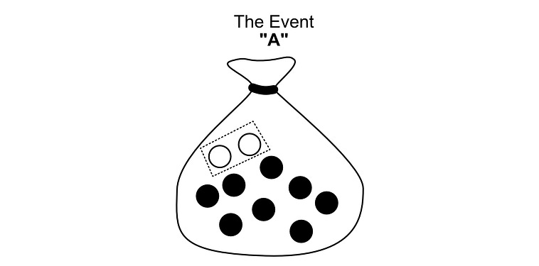
Imagine you have 10 pebbles in a bag. Two of them are white, the rest are black.
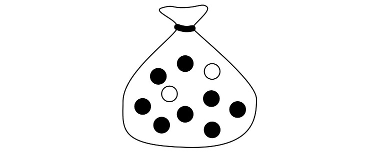
If you randomly select a pebble from this bag, what are the odds it will be a white pebble? There are 10 possible selections, and only two of them are white. So the odds are 2/10 = 0.2 = 20%. We can come to the same conclusion using the definition highlighted above, but to talk about it we need to define a few key words.
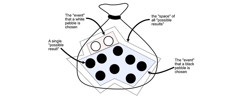
In probability, each pebble is referred to as a possible “outcome”. An outcome is a single result that is possible (i.e. choosing a particular pebble).
A subset of outcomes is called an “Event”. The “event that we choose a white pebble” would be the subset of outcomes that correspond to a white pebble.
The “space” is all possible outcomes. No matter which pebble we choose, we will choose one of the pebbles in the bag.

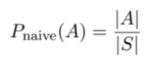
Looking back at our definition, we can see |A|, and |S|.

A naive definition of probability. Source: Introduction to Probability by Jessica Hwang and Joseph K. Blitzstein In our pebble world,
SandArepresents “sets”, a set being a group of possible outcomes.Sis the set consisting of all pebbles in the bag, a.k.a. the sample space.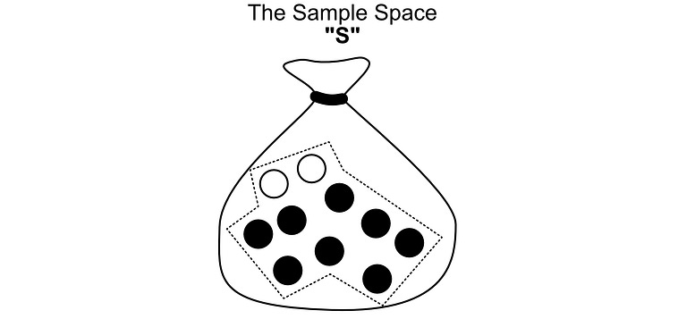
and
Ais the set consisting of just the white pebbles in the bag, a.k.a. the event that the pebble is white.


The vertical bars around each of the sets is a math symbol for “the size of the set”. Here, the size of the set S is 10, and the size of the set A is 2.
P_naive is a function that we’re making that is being applied to a set. So, you would read this expression

as “We’re defining what it means to calculate the naive probability of an outcome in event A actually happening. We’re defining it as the number of outcomes in set A, divided by all of the outcomes in the sample space”.
The issue, and the reason for this article, is that it’s not always easy to count how many possible outcomes there are in the space S, nor how many outcomes are in the event A. For instance, imagine we wanted to calculate the probability that we had a winning hand in poker. To do that, we would need to count how many possible outcomes there were to our poker game, and how many of those games resulted in us winning. Give it a shot, it’s not so easy.
Combinatorics is the study of counting; not counting sheep on a hillside, but the number of combinations, permutations, and arrangements there are in complicated systems. If we count things properly, it’s often easy to calculate probability. The counting is often the hard part.
There are a lot of ways to count things, but in this article we’ll discuss some of the most important ideas as they relate to probability.
Sampling With Replacement
Back to our pebble example.

Let’s ask ourselves two questions.
“If you take a pebble out of the bag, put it back in, shake it, then take another pebble out, what are the odds that it will be white both times”?
“If you take a pebble out of the bag, then take another pebble out of the bag (so you’ve taken two pebbles out of the bag), what are the odds that both of them will be white”?
These are two subtly different problems. The first is called “sampling with replacement”, the second is called “sampling without replacement”. The distinction concerns whether you put the previous pebble back in the bag before choosing a new one.
Let’s answer each of these questions by counting the possible number of outcomes. We’ll start with sampling with replacement:
Question 1
If you take a pebble out of the bag, put it back in, shake it, then take another pebble out, what are the odds that it will be white both times? There are 2 white pebbles, and 8 black pebbles in the bag.
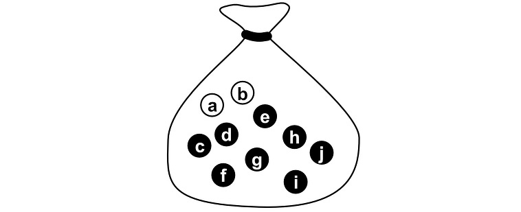
There are several famous examples of many brilliant minds throughout history messing up problems that are similar to this one. To prevent these types of mistakes, it’s often best to give each possible outcome in the space a label.
The end goal is to calculate P_naive(A), where A represents the set of all winning outcomes, and S represents the set of all possible outcomes.

A naive definition of probability. Source: Introduction to Probability by Jessica Hwang and Joseph K. Blitzstein
To ground this in our example, which asks how likely it would be if both the pebbles we took out of the bag were white, A would represent all the scenarios where both pebbles could be white, and S represents all possible selections of two pebbles.
We can start with counting the set of all winning scenarios “A”. There are four possible winning outcomes.
We choose pebble a, then pebble b
We choose pebble b, then pebble a
We choose pebble b, then pebble b again
We choose pebble a, then pebble a again.
Recall, we can choose a pebble twice because we are replacing the pebble into the bag before making our next selection.
So, the number of winning combinations is 4. More formally, the “size of the event A is 4”, and in equivalent mathematical shorthand; |A| = 4. Now we need to calculate the number of possible outcomes, more formally, “the size of the sample space”, or in mathematical shorthand |S|
This is going to be hard to do element by element. Instead, we can use “the multiplication rule”. There are some unintuitive math definitions, but I find a picture speaks 1,000 words. If we have 10 pebbles, we can put all the pebbles in a row, and all the pebbles again in a column.
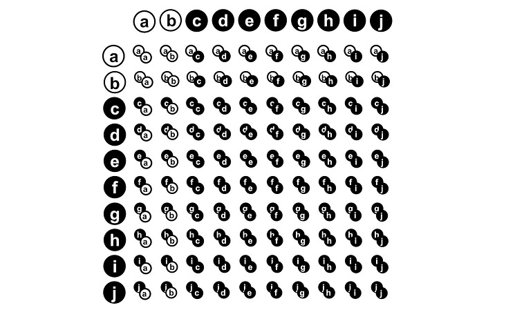
The number of results possible in the scenario of choosing two pebbles out of a bag, after replacing the first pebble before selecting the second, is equal to how many times each pebble can be paired with each other pebble (including itself), which is 10x10. So, there are 100 possible results in the space S.
The multiplication rule describes how many ways one set of things can be combined with another set of things, which we’ll be exploring throughout a few of the example problems in this section.
Earlier, we calculated how many winning possibilities there were, |A| = 4 , and we just counted how many total possibilities there are, |S| = 100, so the probability of choosing two white pebbles (event A) is P(A) = |A|/|S| = 4/100 = 0.04 = 4%
In a way, you can conceptualize this as simplifying the problem. Instead of choosing two pebbles out of a bag of 10 twice, we changed the problem to choosing one pebble out of a bag of 100, where each of the pebbles represents one of the possible pairs.
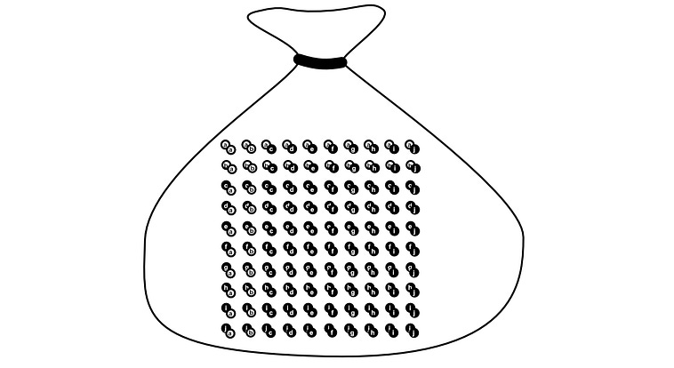
Re framing the problem, as choosing a pair out of all of the possible pairs. Here, the winning event A is not a single pebble, but a pair of pebbles selected which are both white. By counting the number of winning solutions, and the total number of solutions, it’s like we abstracted the problem to choosing a single pebble.
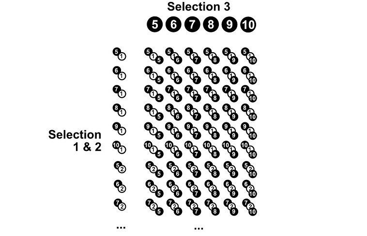
Often, many probability problems turn into “choose k things within a space of N possible choices, with replacement”. Assuming we’re taking k samples from a space of N things with replacement, then there are N^k possible outcomes in the space. We just keep multiplying N for each of the k selections we’re making. If there are 10 things and we’re sampling 3 times, there are 10 x 10 x 10 = 10³ possible outcomes.
This was a pretty simple problem because counting the size of the event A was trivially easy. As previously mentioned, actually counting this can be tricky. To get a hang of this, we can go through another example.
Question 2
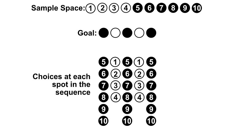
Let’s say we have 4 white pebbles, 6 black pebbles, and we’re selecting 5 times with replacement. What are the odds that we get alternating white and black pebbles? The alternation can start with black, or white.
One might think this problem is simple. There are only two valid resulting sequences. Here, b represents black and w represents white.
[b,w,b,w,b] and [w,b,w,b,w]
So, one might think |A| = 2. However, there are 4 white pebbles and 6 black pebbles, so there are actually numerous selections that can lead to each of these two sequences. Considering each selected object as having a label is important for avoiding these types of issues.
For instance, if pebbles 1, 2, 3, 4 are white, and 5, 6, 7, 8, 9, 10 are black, here is a subset of the sequences which would be valid alternations of black and white.
[5, 1, 5, 1, 5]
[5, 1, 5, 1, 6]
[5, 1, 6, 3, 9]
[4, 9, 3, 5, 2]
...
The trick of this task is counting how many of such valid combinations there are.
The easiest way to solve this problem is to consider each winning sequence separately. We can calculate the number of ways to create a [b,w,b,w,b] sequence, and the number of ways to make a [w,b,w,b,w] sequence. If we add those together, that will be the total number of winning sequences.
Let’s start with sequences starting with black. In the first spot there are 6 valid pebbles, in the second there are 4 possible pebbles, in the third there are 6, fourth there are 4, and fifth there are 6.
[b,w,b,w,b] based on the pebbles we have.We can use the multiplication rule to calculate how many results are possible in this subset. First, we find how many combinations of the first two selections there are
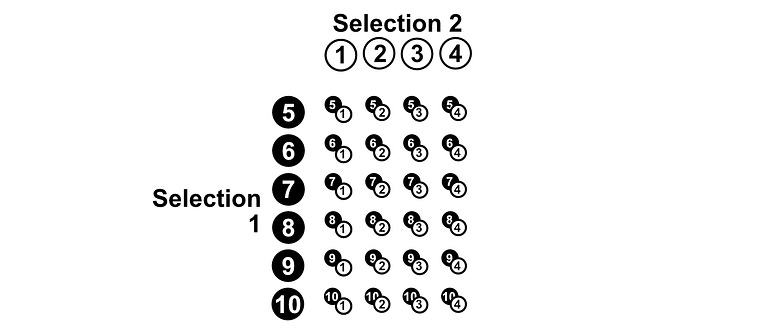
We can use the multiplication rule to figure out how many combinations there are of the first two selections.
then how many ways that can combine with the second selection

We can further leverage the multiplication rule by combining the number of combinations of the first and second selection with the number of possible third selections to count the number of possibilities for the first three selections.
etc, until we’ve calculated all possible sequences. At the end of the day, we calculate that by just multiplying everything together.
6 * 4 * 6 * 4 * 6 = 3456We can do the same things with sequences that start with white squares, using a similar logic.
4 * 6 * 4 * 6 * 4 = 2304If we add those numbers together, we get 3456 + 2304 = 5760possible winning sequences that have alternating colors. Therefore, |A|=5760
Next, we need to count all sequences possible. We can use the same logic, but now there are 10 selections in each spot (all of the pebbles are possible to be selected in each spot). So, 10 x 10 x 10 x 10 x 10 = 100000, so |S| = 100,000
Now that we’ve counted the number of possible winning sequences, and the number of sequences possible, we can use those in our formula to calculate the probability of event A happening (event A being a sequence of 5 rocks randomly pulled from the bag with replacement, being in alternating order of white and black).
P_naive(A) = |A|/|S| = 5760/100,000 = 0.057 = 5.7%
There are some nasty questions you could ask about this situation that require more complicated approaches to counting. We’ll cover some more tools around that later, but for now I think we sufficiently understand the idea of sampling with replacement. Let’s move onto an alternative approach to sampling stones out of our bag.
Sampling Without Replacement
Sampling without replacement is a very similar problem to sampling with replacement, save one key difference; in sampling without replacement, when you take a pebble out of the bag, you don’t put it back in before selecting the next one.
A good first question to ask is “how many possible results are there in sampling without replacement?” If we had, let’s say, 10 pebbles, how many possible sequences could you make by randomly taking pebbles out of the bag, and placing them in a row one after another?
In the first selection there would be 10 possible pebbles to choose from. In the next one, there would be one less, so 9. In the next selection there would be one less, so 8. etc. We can use the multiplication rule we used previously to combine those together and calculate the total number of possible sequences.
If there are 10 possible first stones, and 9 possible next stones, then there are 10 * 9 = 90 possibilities for our first two stones. There are 8 possible third stones, which we can combine with our 90 possibilities for the first two stones, to get 90 * 8 = 720 possibilities for the first three stones.
You might be able to read between the lines, but there are 10 * 9 * 8 * 7 * 6 * 5 * 4 * 3 * 2 * 1 = 3,628,800 possible outcomes when sampling 10 stones out of a bag without replacement. This idea of multiplying the subtraction of one less than a number until you hit 1 is pretty common, which is why it’s often denoted with the symbol !, which stands for “factorial”. 3! = 3*2*1 = 6 , or 5! = 5*4*3*2*1 = 120 , for instance. 3! counts how many ways you can choose a sequence out of three things without replacement, and 5! counts how many ways you can choose a sequence out of five things with replacement. These both assume you’re selecting all of the elements from the set. If you’re selecting a specific number of things, say 4 things out of a bag of 10, you would do 10 * 9 * 8 * 7, stopping after you got to the 4th selection.
Just like sampling with replacement, calculating how many possible results exist within event A is sometimes easy, and sometimes hard. It takes some practice to get good at it, so let’s try another problem
Question 3
Six students line up randomly; Alice, Bob, Joyce, Tom, Nancy, and Daniel. What is the probability that Alice and Bob stand next to each other?
It’s not possible for Bob to be standing next to Bob, there’s only one Bob. Thus, this is a classic sampling without replacement problem. There are six people, which means there are 6! = 6 * 5 * 4 * 3 * 2 * 1 = 720 possible ways we could line these people up in a line, meaning |S|=720 in this example. To calculate the probability of Bob standing next to Alice, we need to count how many of those possible sequences include Bob and Alice sitting next to each other. To do that, we can use an approach called the “blocking” method.
There are two characteristics of a sequence that can make it valid; if the sequence has Alice, Bob in the sequence, or if the sequence contains Bob, Alice. It doesn’t matter where in the sequence these are, just as long as one of these two sub-sequences exists within the sequence, it’s a winning sequence.
Let’s consider one of those sub-sequences for now. We need to count how many possible ways there are for Alice, Bob to exist within the greater sequence. In other words, how many ways can we stick (Alice, Bob) into a sequence that also contains Joyce, Tom, Nancy, and Daniel. To do this , we can treat the sub-sequence (Alice, Bob) as a single block which gets selected just like any of the other names. after we combine Alice and Bob into a single unit, there are 5 things, meaning there are 5! = 5 * 4 * 3 * 2 * 1 = 120 ways to arrange (Alice, Bob), Joyce, Tom, Nancy, and Daniel. The act of treating multiple selections as a single “block” is the namesake for the “blocking” method of counting.
By the same logic, there are 120 other ways to create sequences that has (Bob, Alice), so in total there are 240 possible and equally likely sequences where Bob and Alice end up standing next to each other. Because there are 720 possible sequences, that means there’s a |A|/|S| = 240/720 = 33% chance that the two will be standing next to one another.
There’s a subtlety that I think is important to address; in this example, we care about the number of ways to order the sequence. All of the sequences have the same set of people in them, but we’re counting how many ways we can arrange that set. Let’s cover a different but very common flavor of question in the sampling without replacement space, where we don’t care about the order of the result.
N Choose K
Let’s take our previous people, Alice, Bob, Joyce, Tom, Nancy, and Daniel. How can we make a random committee of three people? Or, in other words, how many ways are there to select three people out of our six possible people in this scenario? It’s important to note, in this scenario, we don’t care who was chosen first, only what committee was chosen. So, the selection (Alice, Bob, Joyce) is treated as the same result as (Joyce, Bob, Alice).
This problem, and problems like it, are solved using “N choose K”, also known as the “Binomial Coefficient”, a very common approach to counting that’s helpful when you need to count how many ways some number of element (K) among a larger number of elements (N) can be selected in a “sampling without replacement” manner.
We can actually derive the formula for “n choose k” ourselves with a little bit of pondering and eyebrow furrowing. There are several ways to come up with a formula for “n choose k”, I’m partial to using an approach called “adjusting for overcounting”.
The essential idea is that you can adjust for over-counting things if you know exactly how many times you over-counted. If you put five pennies on a table, count each of them twice, then divide by two, you would get five pennies. Obviously this is a bit silly, but sometimes it’s easier to calculate some multiple of something, then adjust by that multiple.
In our committee example, a committee of Bob, Joyce, Tom should be considered the same as Tom, Bob, Joyce. Let’s put that to the side for a moment and count how many three person sequences are possible, where different orders of people are treated as different outcomes. We’ve already explored the answer to this question, it’s just like taking three stone out of a bag without replacement. There are 6 names, so there are 6 * 5 * 4 = 120 possible ways to make sequences of three names out of the possible 6. This won’t tell us how many committees there are, because that 120 number contains both Bob, Joyce, Tom and Tom, Bob, Joyce. Each committee is represented some number of times within that 120 number. The question is, how many times?
Well, we know how many ways three people can be represented as a sequence. If we had three names, Tom, Bob, and Joyce for instance, We could represent those people in 3! different sequences, 3! = 3 * 2 * 1 = 6.
So, we know how many sequences of three names are possible out of all of the names, 120, and we know that each three person committee is represented 6 times within that number (because there are 3!=6 ways of expressing 3 people as an ordered sequence). To calculate the total number of committees, we can simply divide 120/6 = 20, effectively adjusting for the fact that we counted our committees too often when we counted the number of possible ordered sequences of length 3.
Because “n choose k” is so widely used, it has a variety of shorthand representations in mathematics.
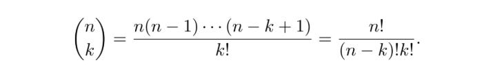
Three representations of n choose k. Source: Introduction to Probability by Jessica Hwang and Joseph K. Blitzstein
The definition in the middle is the one we came up with. If you have n things, and you want to choose k sequences from that set of things, you can do that n * n-1 * n-2 * ... * n-k+1 ways. That will include counting the same group in a different order as a different result. If you want to adjust for that, and only count the number of ordered sets possible, you divide by k!.
To the left of our definition is the common shorthand for “n choose k”. When you see a number over another number between parentheses like that, in a probability and statistics context, then that means “n choose k”. It’s so common it gets it’s own fun math representation.
Over to the right is an algebraically equivalent, but slightly more convenient definition of “n choose k”, which you can plug right into a calculator.
The one on the left is convenient shorthand, the one in the middle is the most conceptually simple, and the one on the right is the most mathematically convenient. They all represent the same thing, n choose k, also occasionally referred to as the “Binomial Coefficient”.
Now that we understand the general idea, we can use concepts of “n choose k” to solve all manner of problems. We’ll start with a softball question, and then ramp up our understanding.
Question 3
You and your 10 colleagues are on the board of directors. A committee of three people is being randomly formed. What is the probability that you will be on the committee?
First of all, to figure out the probability of some event A happening ( A representing all the results which include you on the board of directors), we can use the equation P(A) = |A|/|S| (The probability of A happening is the size of event A divided by the size of the entire sample space), which we’ve used a few times now. To do that, we’ll need to calculate the size of event A, and the size of the sample space S.
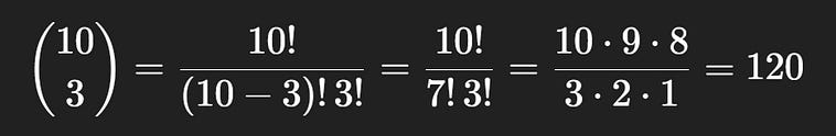
S, in this context, represents all of the possible committees that can be created. We can calculate the size of this space easily using our newfound knowledge of “n choose k”. In a group of 10 people, a committee of 3 can be chosen 120 different ways.

10 choose 3, the total possible number of committees.
Now we need to calculate the size of space A, which represents all possible ways a committee can be created where you are a member. We can calculate this easily with a bit of mental tai chi. If we’re a member, then the committee will always include us. So, another way to ask “how many possible committees contain me” would be “how many ways could we complete a committee, assuming I was already selected”.
If we’re already a known member, then we would need to find how many committees of 2 can be created from the remaining 9 people. To do that, we can just use “n choose k” again.

9 choose 2, the total number of committees where you are a member.
So, 10 choose 3 represents the total number of possible committees, 120 , and 9 choose 2 represents the total number of committees where you are a member, 36.
P(A) = |A|/|S| = 36/120 = 0.3 = 30%Thus, the probability that you will be a member of the committee is 30%. Repetition brings mastery; let’s do another.
Question 4
You have a bag with 10 pebbles. 4 are red, 6 are blue. You randomly select 3 pebbles in one handful. What is the probability that exactly two of the pebbles are red?
Based on what we know so far, this is a bit of a trick question. We’ve done sampling with and without replacement, but never conceptualized what it means to grab a handful of rocks out of a bag.
As humans, it’s common for us to give order to things, and to conceptualize things based on that order. I’m going to clean the house, which means I’m going to clean the living room, bathroom, kitchen, bedroom, my shrine to Rihanna, and the dining room. Simply by listing those things in that order, we naturally decide that the plan must be to clean the things in that order, but cleaning in any other order would be the same result.
In some sampling without replacement problems, we care about order. If we take black and white rocks out of a bag, we might decide that the sequence white, black, white, black should be counted as a difference result than the sequence white, white, black, black. Then again, we might not care about the distinction. It depends on the context of the question. When we grab a handful of pebbles out of the bag, we are sampling without replacement, without regard to the order of the sequence. When we grab three stones, we’re not sure which stones we’ll get, and there’s no concept of order, but we do know we won’t get the same stone twice.
“n choose k” Also does not care about the order of the sequence, only that the elements in the sequence are mutually exclusive. That is, you can’t pick the same stone twice. This can be conceptualized as choosing the first person then the next two people (like in our committee example), or it can be conceptualized from back to front (like if you were counting how many ways the winners could be arranged in a race when you know some number already lost), or you can disregard the concept of order entirely and just grab a handful of pebbles out of the bag. The concept of order can be helpful in rationalizing a problem, but because “n choose k” is adjusted to account for how many orderings there are of k things, it doesn’t care about order at all.

Recall the whole point of n choose k. We want to know how many committees of k people can be chosen out of n people. The same committee, chosen in a different order, is still the same committee. Recall that we derived the middle definition of the function by representing the top as how many possible k sequences could be constructed out of the n options, then we divided by the number of ways a sequence of k things can be written. Thus, we adjusted our count to compensate for the fact that we had several versions of each committee, but in different orders. Source: Introduction to Probability by Jessica Hwang and Joseph K. Blitzstein
So, we can happily apply “n choose k” to grabbing three pebbles out of a bag, or we could re-frame the problem conceptually as choosing three stones one by one, then employ “n choose k” in that context, or we could get weird and imagine choosing the last stone, the middle stone, then the first stone. The math would be the same regardless of how you conceptualize the problem.
There are examples where you can’t disregard order, like in environments where choices are not mutually independent. Choosing to buy a drink, then a straw, might not be mutually independent choices (you probably bought the straw because you bought the drink), so we would probably want to consider their order in some way. We’ll discuss those types of problems later. In this problem, choosing one pebble doesn’t make you any more or less likely to choose some other pebble in particular, so we can disregard order.
Anywho, back to the task at hand. To calculate the possibility of choosing exactly two red marbles and one blue one, which we’ll call event A, we can use the naive definition of probability, p_naive(A) = |A|/|S|. So, like usual, we need to count out how many results are in event A, and in the space S.
|S| is straightforward, provided you understand the idea that n choose k doesn’t care about order. If you want to select 3 pebbles out of the possible 10, there are 10 choose 3 possible ways to do it.
So, |S| = 120 .
Now we need to count how many ways we could choose two red pebbles and one blue pebble. In other words, we need to figure out how many ways we could choose two red pebbles out of the four red pebbles in the bag, and combine that with the number of ways we could select one blue pebble out of the possible six blue pebbles.
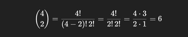
We can calculate each of those independently fairly easily. There are 4 choose 2 ways to choose the two red pebbles we need out of the four in the bag, and there are 6 choose 1 ways to choose the remaining blue pebble.
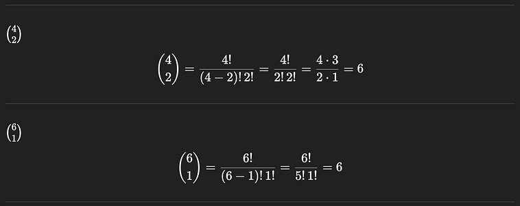
4 choose 2, and 6 choose 1, respectively.
To calculate |A|, we need to calculate the total number of ways two red pebbles could be chosen in our handful of three. To do that, we can use the multiplication rule we discussed previously. There are 6 ways to choose the two red pebbles, and 6 ways to choose one blue pebble, so there are 6 * 6 = 36 possible ways to choose exactly two red pebbles in a handful of three, in this scenario. Thus, |A| = 36.
If you’re like me, this might make logical sense, but not feel intuitive. We’re going for a thorough understanding here, so “I’m following you” isn’t sufficient. If you’re still confused, here’s a description that may be slightly more intuitive.
Keep in mind, in figuring out the size of the event A, we’re counting all the possible ways we could have a set of three pebbles with two red stones and one blue stone. We don’t care about order, there isn’t even a concept of order implicit to this problem, but there are a certain number of red and blue stones in the bag. If we had 10,000 blue stones, and 2 red stones, it would be very unlikely for us to get our two red one blue combo, because pulling out the 2 red stones would be very unlikely. Also, if we had 10,000 red stones and 1 blue stone, it would also be unlikely for us to get a handful consisting of two red and one blue. Regardless of the approach, intuitively, we need to account for how many stones of each type there are. Recall, a good way to do that is by assigning each stone in the bag with a label. If we had red pebble 1, 2, 3, … 10,000, then there are 10,000 different ways we can pull out a red pebble.
Regardless of the sequence we’re going for, this is also useful to keep in mind; no one stone is more likely to be pulled than any other stone. If we had 10,000 red stones and 1 blue stone, you would be 10,000x more likely to to pull out a red stone. This isn’t because one of the red stones is very likely to be pulled, but because there are more red stones than blue stones. It is equally likely that you would pull the blue stone as it would be for you to pull red stone #6, for instance. Every stone is just as likely as any other. The event of pulling a red stone is more likely than the event of pulling out a blue stone because the event of pulling out a red stone consists of 10,000 possible results, and the event of pulling out a blue stone only consists of the one.
By the same logic, if we go back to pulling out a handful of three stones, any handful is just as likely as any other. You are just as likely to pull stones #1, #3, #5 as you are to pull stones #1, #2, #3, for instance. The reason you are more likely to pull some collection of red and blue stones is because there are multiple red and blue stones. Because any collection of individual stones is equally likely, we can calculate the probability of pulling two red stones and one blue stone by finding the percentage of winning handfuls there are, which is what |A| / |S| represents. This idea of equally likely things is super important, and we’ll revisit it later in the article.
Counting |S| as 10 choose 3 hopefully feels fairly intuitive. We care about unordered sets, not ordered sequences, and n choose k allows us to count how many ordered sequences of k things there are, divided by how many ways there are to arrange k things, thus giving us how many unique unordered sets of 3 can be created from the 10 pebbles.
Counting |A| is more intuitively complicated, but keep in mind what it represents; the total number of possible sets of pebbles #1, #2, #3, #4, #5, #6, #7, #8, #9, #10 that would have two red and one blue pebble.
It stands to reason that the total number of possible 2 red and 1 blue sets would be equal to the number of 2 red sets possible times the number of 1 blue sets possible. Imagine if we could lay out all the ways we could get 2 red pebbles vertically, and all the ways we could get 1 blue pebble horizontally. The height of that square, times the width, would be the number of possible ways to get 2 red squares and 1 blue square. That’s why the multiplication rule works in this scenario.
Recall, in a previous example, we combined the number of ways two things could be combined, with the number of selections for another thing, to get the total number of possible selected sequences. We can use a similar intuition to combine the number of ways to get two red stones, times the number of ways to get one blue stone, to get us the number of ways we can get two red and one blue stone.
So, the question then becomes, how many ways are there to get 2 red pebbles, and how many ways are there to get 1 blue pebble. The second question is trivial to answer; there are 6 blue pebbles, so there are 6 ways to select a blue pebble from the bag. I think the only conceptual hang-up here might be something along the lines of “but wait, there are other pebbles, red ones!” But we don’t care about those in this part of the answer. We’re counting how many ways there are to create a winning hand, which means calculating how many ways there are to get a blue pebble.
Similarly, in counting how many ways there are to get two red pebbles, we don’t care that there are blue pebbles in the bag. We account for that in other parts of the answer. To help us count the number of winning hands, we need to count how many ways we can get two red pebbles. When the context is properly framed, the answer is obvious; to get 2 red pebbles out of the 4 that exist in the bag, there are 4 choose 2 ways to do it, which is equal to 6.
So, we’ve counted how many ways there are to get 1 blue pebble, 6 different ways, and we’ve counted how many ways there are to get the two red pebbles, 6 different ways. We can multiply those together, and conclude that there are 6 x 6 = 36 possible winning handfuls of pebbles. That’s our |A|, the size of the event A in which we have a winning hand.
In probability, it’s easy to make mistakes. Not because the math is hard, but because the concepts can be slippery, and misconceptions are common. It’s worth the time to try to really think through a problem.
Regardless, we’ve established that |A| = 36, and earlier we established that |S| = 120. So, the probability of a handful of pebbles having two red and one blue in this scenario is P_naive(A) = |A|/|S| = 36/120 = 0.3 = 30%.
n choose k is used in a huge number of disciplines; mastering all its subtle uses is outside of the scope of this particular article. Rest assured, though, I will be reviewing it often in future articles on probability. For now, I want to cover a few more topics before we wrap up.
Complete and Partial Permutations
We’ve already covered the likely suspects of combinatorics from a probability perspective, but I wanted to cover a few more dangling concepts.
A “permutation” is a way you can organize things. If we have the set of numbers {1, 2, 3}, they could be represented as the ordered sequence (1,2,3), or (3,2,1), for instance. Each of these would be called a “permutation” of the set {1, 2, 3}.
Permutation can also be used as a verb, “Permute” or “permuted”, which means to generate all the permutations possible from a set of numbers. The numbers 1, 2, and 3 can be “permuted ” in the following ways:
(1, 2, 3)
(1, 3, 2)
(2, 1, 3)
(2, 3, 1)
(3, 1, 2)
(3, 2, 1)
We’ve encountered this under another name: sampling without replacement. When you take pebbles out of a bag, one by one, without replacement, you are making an ordered sequence out of a set of possible outcomes. Finding the number of possibilities in a sampling without replacement problem is the same as finding the number of permutations of that set.
As we previously discussed, the number of results you can get by sampling all pebbles out of a bag without replacement is n! (n x (n-1) x (n-2) x … x 1). Counting the number of permutations is the same thing, and thus has the same mathematical definition.
There’s another type of permutation, called a partial permutation, which we’ve also discussed; It’s how to make some number of ordered sequences that is smaller than the total number of selections available. For instance, we can find the number of partial permutations of length 2 which we can generate out of our set of choices {1, 2, 3}:
(1,2)
(1,3)
(2,1)
(2,3)
(3,1)
(3,2)
Interestingly, there are six of them; the same number as the number of full permutations. That’s a complete coincidence, usually the number is different.
There are numerous ways partial permutations are notated in math

several different and valid ways partial permutations are notated.
The most common is P(n,k), where P denotes “permutation”. Naturally, this can get confusing as we already have a very important “P”, which denotes probability. Thus, the other notations are sometimes used.
We’ve discussed how to calculate a partial permutation. If you have 20 things, and you want to calculate the number of ways you could select ordered sequences of length 3 from that set, it would be 20 x 19 x 18 = 6,640 possible ways. In other words, there are 6,640 partial permutations of length 3 that are possible when selecting from a space of 20 possible events.
If you look at math textbooks you might see the following formula used to describe partial permutations:

This is calculating the number of partial permutations, but by way of a slightly different conceptual path than we’ve discussed. It uses the idea of adjusting for overcounting.
Let’s imagine we had the set {1,2,3,4,5}. Let’s generate a single permutation, and a single partial permutation of this sequence. Let’s use a partial permutation of length 2 for this example.
permutation:
(5,1,2,4,3)

length-2 partial permutation:
(5,1)
As you can see, in this example, the partial permutation of length 2 is a subset of the full permutation.
You can re-frame this question. Instead of asking “how many partial permutations are there of length 2 ”, you could say “how many full permutations exist which start with (5,1)”.
If you took 5 and 1 out of the set, you would have these remaining numbers:
{2,3,4}And there are 3! ways of organizing these three numbers into a sequence (a.k.a, 3! permutations of this set). Thus, there are 3! ways these numbers can be tacked onto (5,1) that would result in a unique sequence. That’s not just the case for the sequence of (5,1); for any sub-sequence of length 2, there are 3! permutations that will start with that sequence in the space of all possible full-length permutations.
Thus, to answer the question of “how many partial-permutations of length 2 are possible”, we can count the total number of full permutations possible (5!) and correct that by dividing it for the fact that there are 3! (n-k)!) full length permutations for each partial permutation. Thus, the mathematical definition of the number of partial permutations:
Let’s cement our understanding of the idea with a question.
Question 5
You have 5 distinct books labeled A, B, C, D, and E. You randomly arrange 3 of the books on a shelf, in order. What is the probability that book A is first and book B is second?
We actually have the ability to solve this problem without the concept of a permutation. We solved a very similar problem in Question 3, where we tried to find the number of ways Alice and Bob might sit next to each other. Partial permutations are simply a named idea which we can use to help us solve this type of problem with less brainpower.
Recall the naive definition of probability; P_naive(A) = |A|/|S|. We simply need to calculate the number of ways the event A can happen (book A is first and book B is second in the three spots), divided by the size of the space of total possibilities S.
Counting |A| is super simple; we know A and B are in spots 1 and 2, so we just need to figure out which books can be in spot 3. There are three remaining books, C, D, and E, so there are three possible sequences where A and B are in spots 1 and 2. thus |A| = 3.
Counting |S| is a bit more complicated, but with a knowledge of partial permutations, we don’t need to think through the logic from bedrock. We have books A, B, C, D, and E; 5 possible choices. We need to figure out how many unique ordered sequences can be created by putting them into 3 spots. That’s the textbook definition of a partial permutation where n=5 and k=3. Thus, we can count |S| by using the partial permutation formula.

So, |A|=3 and |S|=60 . That means P_naive(A) = 3/60 = 0.05 = 5%.
Complements and Derangements
Another important concept I want to cover is the idea of a complement.
In math speak, a complement of an event is all of the possible results that do not fall within that event, but are in the sample space. If you have a rock-solid intuition of an “event” as a set of possible outcomes this should be intuitive, but the verbiage of probability has a way of making simple concepts confusing.
Using an example to hopefully cement the idea of a complement; if we had a bag of pebbles, we could define event A as if we selected pebbles #1, #2, or #3. The “complement” of A would be all of the pebbles that are not in event A, so pebbles #4, #5, and #6.
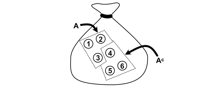
If A is a set, then the complement (denoted as A superscript c) is all other possible results in the sample space.
Complements are incredibly useful in both combinatorics and probability. It’s sometimes easier to calculate the complement of some event and the size of the possible space, rather than the event itself. For example:
Question 6
You take five distinct books off a shelf, shuffle them, then put them back on the shelf. What is the probability that at least one book is in its original position?
You could try to count how many ways one book could be in it’s correct spot, then count how many ways two books could be in the same spot, then three, then four, etc. This is possible, but difficult. Instead, we can solve this problem much more easily by leveraging a simple fact:
The number of ways the books can be arranged on the shelf is equal to the number of ways they can be arranged where at least one is in the correct spot, plus the number of ways they can be arranged where no books are in the correct spot. Doing some linguistic algebra here, you could also say the number of possibilities where one book is in the correct spot is equal to the number of possibilities in total, minus the number of possibilities where no books are in the correct spot.
If we can calculate how many arrangements there are, and how many arrangements do not satisfy the criteria, we can use that information to solve the problem by way of complements.
The size of the space is simply 5!, classic permutation/sampling without replacement problem.
Calculating the number of ways of organizing the books so that none of them are in the same spot… Well… I said it’s easier, but it’s not easy. The idea of shuffling things so that no items are in the same spot is called a “derangement”. A derangement, by definition, is a permutation where no items end up in the same spot.
The number of derangements for n things is written as !n, notice how the exclamation point is in front of, rather than behind the n. n! represents the number of permutations, !n represents the number of derangements.
There’s a formula for the number of derangements, which we could use without any understanding of how it worked if we really wanted to.

The formula for the number of deranagements of a sequence of `n` things.
But, this is IAEE, and derangements are a common topic in combinatorics and probability, so we need to build an intuitive understanding of why this works.
The whole idea of a derangement !n is to count all the ways to arrange a sequence of n things so none of the things end up in the same spot. We can start with the number of permutations, n!, which is all of the ways we can list out the sequence.
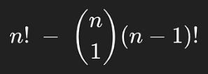
We can then think of this as an overcounting problem. The number of permutations n! includes examples where one of the books is in the right spot, so we want to then subtract from that the number of examples where one of the books is in the right spot. If we want to count the number of ways book 1 can be in spot 1, that would be equal to the number of ways we could arrange all the other books, (n-1)!. One might think this applies to all n books, which means there are n*(n-1)! ways that at least one book could be in the same spot it started. If we subtract that from the total number of permutations, we would account for all of the ways one book being in the right spot is represented in n!
but this is slightly incorrect.
See, imagine a case where there are two books in the same spot they started in. That case would be counted in both of the books (n-1)!‘s, meaning we over subtracted and accounted for that case twice. We can figure out how many groups of two people there are using n choose 2, and multiply that by how many sequences there are to add them back in.

The number of permutations, minus the ways there can be an overlap, plus a correction for over-subtracting instances where there are two books in the correct spot.
But wait, what about permutations where there are three books in the correct spot? Let’s imagine one, where books 1, 2, and 3 are all in the correct spot. We’re trying to count the number of derangements, so a case where books 1, 2 and 3 are in the right place should not exist in the count.
Well, it’s counted once in n!, which it shouldn’t be.
It’s then subtracted three times in the next term; once for the (n-1)! of book 1, of book 2, and of book 3. Keeping in mind it was over counted by 1 previously, means this sequence has now been excessively compensated for by -2.
books 1, 2, and 3 would be counted in situations where two books are in the right spot. In fact, it would be included three times;
for books 1 and 2 being in the right spot
for books 2 and 3 being in the right spot
for books 1 and 3 being in the right spot
So we add +3 to the count for this sequence. Because we under counted by -2 from the previous step, that means in total, across all terms in this expression, sequences of three are over counted by 1, so we need to compensate for that by adding a term which subtracts each sequence of three books in the right spot.

You may be able to read between the lines. This would over compensate correct sequences of 4, then over compensate the other direction for sequences of length 5, etc. etc. Thus the general form of the expression is defined as

or, with some factoring out of n choose k, we get the simpler expression

If you’re not familiar with summation notation, I won’t bore you with the details; our original representation of the equation is more intuitive, which is the same thing just rolled out.
The formula for the number of deranagements of a sequence of `n` things.
You can see we’re starting with n! (which is multiplied by the 1 in the parentheses), then subtracting n!/1!, then adding n!/2!, subtracting n!/3!, and on and so forth until we’ve done that n times. This is the general expression which allows you to do the same intuition we’ve been discussing, but for any sequence of length n.
You might not have a complete understanding of derangements, but that’s ok. These things take practice, and you can review the concept as it comes up. I think what’s most important is that you know what a derangement is, and understand the vague idea of how they’re counted.
So, back to the task at hand, we can now calculate the number of derangements of our five books, it’s
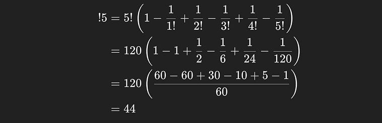
So the number of ways none of the books will end up in their original position is 44.
Recall that the point of the problem is to count how many ways at least one book would end up in its original position. Well, we know how many sequences are possible, |S|=5!=120, and we know how many sequences there are which don’t have any books in the original spot, !5=44, so the number of ways at least one book will be in the original spot is simply |A| = 5! — !5 = 120-44 = 76. Now that we know the number of winning sequences possible, and the size of the whole sample space, we can calculate the probability as P_naive(A) = |A|/|S| = 76/120 = 0.63 = 63%.
Distinguishable and Indistinguishable Things
I’ve mentioned a few times that it’s a good policy to assign labels. If you have 10 people, and you need to make a committee of 3, it’s a good idea to assign names or numbers to each of the people so you correctly conceptualize the problem.
In some situations, identifying what is distinguishable is easy. We have 10 people, give them a name. Sometimes assigning labels is a bit more counterintuitive. Take the following example:
Question 7
You have 5 balls and 3 boxes. In how many different ways can you distribute the balls among the boxes?
You can decide to label the balls and sample the boxes which the ball is in, you can decide to label the boxes and sample the balls that land in them. There are various ways you can wrap your head around this problem.
We can look at a slightly different wording of the problem, which has a big impact:
Question 8
You have 5 identical balls and 3 boxes. In how many different ways can you distribute the balls among the boxes?
The word “identical” means that results should be treated as the same if ball A ended up in box 1 , or if ball B ended up in box 1. By saying the balls are identical, we’re saying we don’t care which ball ends up in a box, so long as a ball ends up in the box. This changes how we would count.
This type of problem comes up occasionally in probability, and requires a slightly different mental model to count effectively. When you have buckets of indistinguishable things, often the “stars and bars” approach is used.
We can model our problem as a series of stars and bars. The bars represent where we transition from bin 1 to bin 2, or bin 2 to bin 3. Here’s an example:
* * | * | * *In this example of the notation, we’re saying two balls ended up in the first bin, one ended up in the second, and two ended up in the third. In another example:
| | * * * * *We’re saying no balls ended up in the first and second buckets, and they all ended up in the third bucket. Using the stars and bars as a modeling tool is useful because it allows you to visualize how these indistinguishable things might end up in distinguishable places.
When using the stars and bars, the next intuition becomes slightly more obvious; To count how many different ways our identical balls can be distributed across bins, we just need to count how many ways we can position our bars within the stars. In this example, there are 7 total positions the bars can be, which is the total number of stars plus the number of bars (the number of bars being the number of buckets minus 1, so 5 + 3–1).
* * | * | * *
1 2 3 4 5 6 7
We need to choose which of these 7 locations one of our two bars falls into. Here, the bars are treated identically; there is no bar “a” and bar “b”, the bar on the left always means the transition from the first bin to the second, and the second bar always means the transition from the second to the third bin. So, to count how many distributions of balls we can have within boxes, we need to choose how many unordered sets of two numbers can be chosen from the set {1, 2, 3, 4, 5, 6, 7}. As you may recall, that’s n choose k.

So, the number of possible distributions of five identical balls in three boxes is 21.
I saved this for the end of the article because the way it relates with probability is kind of sneaky. In this problem, we’re not coming up with any probabilistic claims about the sequences, we’re simply counting how many possible distributions of balls within boxes are possible. Just because we counted 21 things doesn’t mean each of those 21 things is equally likely.
One could say that, if there are 21 possible distributions, each of those possibilities would have a 1/21 chance of happening. One could also say that, if there are eight planets in the solar system, and one of them has life, then each of them has a 1/8 chance of having life. Just because you have some number of things doesn’t mean they have equal probability.
Recall the naive definition of probability we’ve been using
We’ll discuss this at more length in future installments, but a big reason this is naive is because it assumes that all of the possible outcomes are equally probable, which isn’t always the case.
We were told we have 5 identical balls, which was important for counting how many distributions of those identical balls are possible in the three boxes. However, if we tried to calculate the probability of one distribution or another, assuming the balls might land in each box with equal probability, it’s obvious that a distribution like this:
| | * * * * *is less likely than a distribution like this
* * | * | * *There’s only one way to create the first distribution, but there are 30 ways to create the second

For the second sequences, two of the five balls land in the first box, and one of the remaining balls lands in the second box. Multiplying these together yields the total number of possible ways this distribution could be created.
any specific distribution of labeled balls in boxes is just as probable as any other, but there are 30 of them that can represent * * | * | * *, while only one can represent | | * * * * *. Sometimes the verbiage of probability can make understanding it difficult. The stars and bars approach is very uncommon in probability, because it’s very uncommon that each of the distributions is actually equally likely. Typically, when trying to make probabilistic claims, it’s best to treat each thing you’re selecting as unique, even if it isn’t.
For the sake of thoroughness, there is another flavor of this type of problem, where both the balls and boxes are considered identical.
Question 9
You have 5 identical balls and 3 identical boxes. In how many different ways can you distribute the balls among the boxes?
The math for this is a bit more complex, and it’s application is even less common than stars and bars, so we won’t go over this in depth. To be brief, though, this is called a “partitioning” problem. We want to figure out how many ways there are to divide up the 5 balls. In this example, there are 5 ways
5
4 + 1
3 + 2
3 + 1 + 1
2 + 2 + 1
Again, if you’re chucking balls into boxes, then each of these partitions is not equally likely. While this falls within “combinatorics”, the study of counting things, it’s not often relevant to probability.
I think there’s a general lesson we can take away from this section. Just because you can count things doesn’t mean each thing is equally probable. When making probabilistic claims, it’s useful to label things, and to spend some time making sure the things you’re counting are equally likely. That will make coming to terms about probabilistic claims easier. We’ll explore that general theme in future articles. For now, I’d like to cover one more topic before we close out our discussion of combinatorics for probability.
Counting by Category
We’ve already discussed this topic, but I want to take some time to cement it as a concept.
Recall the idea of the multiplication rule. If you have some number of possibilities of one thing, and some number of possibilities of another thing, you can multiply those numbers together to get the total number of possibilities.

Recall the multiplication rule
Based on the previous section, you might have some suspicions about if each of those combinations is equally likely, which is a great intuition. When making probabilistic claims in the real world, that’s very important to keep in consideration.
Assuming certain combinations aren’t especially privileged, there’s a useful way of conceptualizing these problems in complex situations, which is to use “counting by category”. Essentially, you can divide the problem in to categories of things, then combine the counts of the categories together.
Rather than be theoretical, let’s use an example.
Question 10
You draw two cards in order from a standard 52-card deck without replacement. What is the probability that the first card is a heart, and the second card is a face card (Jack, Queen, or King of any suit)?
This is a sampling without replacement problem, where we care about the order of the outputs. Because every pair is equally likely, we can use the naive definition of probability P(A)=|A|/|S|. Counting the size of the possible space is easy, there are 52 possible first choices, and 51 possible second choices, so |S| = 52*51 = 2652.
Now we need to count the size of space |A|, which is a bit more complicated. We can start to make ground on this problem by breaking it into two parts: Counting the number of possibilities for the first card, and counting the number of possibilities for the second card.
For those of you who don’t play a lot of cards, there are 13 heart cards in a standard deck (1, 2, 3, 4, 5, 6, 7, 8, 9, 10, J, K, Q), so there are 13 choices for the first card. What’s tricky, though, is that some of those cards are face cards (the Jack, King, and Queen). If we select those cards in the first spot, then we can’t also select those in the second spot as well. We need to account for that when counting.
To do that, we can divide our count into two subclasses: one where the category of the first card is a numbered heart card, and one where the category of the first card is a face heart card.
If the first card is a numbered card, then there are 12 possible face cards to pick (a Jack, King, or Queen for each of the four suits, clubs, diamonds, spades, and hearts). So, the number of possibilities of choosing a winning hand, assuming the first card was a numbered card, is number_of_numbered_heart_cards * number_of_remaining_face_cards = 10 * 12 = 120
If the first card selected is a face card (the Jack, king, or queen of hearts), then there is one less face card we can select for our second card, so 11 cards. That means, the number of possibilities of choosing a winning hand, assuming the first card was a face card, is number_of_face_heart_cards * number_of_remaining_face_cards = 3 * 11 = 33
So, we’ve counted all the possibilities of winning if the first selection was and was not of the class “face card”. Because each of those classes ultimately considers all possibilities, we can add them together to get our final result.
number of winning posabilites =

number of wining possibilities if the first card is not a face card

+

number of winning possibilities if the first card is a face card

= 120 + 33 = 153
Thus, the size of the solution space |A| = 153 , and therefore P(A) = |A|/|S| = 153/2652 = ~0.06 = ~6%.
This type of problem can come up a lot. For instance, if you have a talent pool where some people are engineers, some people are designers, and some people are both, and you’re trying to make probabilistic claims about creating a team, you’ll need to account for the fact that there may be people that occupy both the class “designer” and “engineer”, like how we accounted for cards that were both face cards and hearts. You might also be dealing with scheduling problems, where certain types of meetings need to occupy certain time slots, but there’s overlap between the classes of meeting types. It’s also used a lot in medicine, where different classes of people (those that do or do not have a disease, for instance) are used to assign probabilistic claims to the rate of effectiveness of a drug.
Getting good at counting by category takes experience and practice, but I think a valuable first step is knowing that the approach exists in the first place.
With that, I think I’ve covered everything I wanted to in this article.
Conclusion
Hopefully you have a stronger intuition of probability just by reading this article. We have yet to dive into the subtleties of probability itself, but for many problems simply being good at counting, and counting the right things, is more than sufficient.
Now that we have a thorough understanding of counting, we can explore probability itself to a greater degree of depth in future installments. Stay tuned, and consider subscribing to intuitively and exhaustively explained. If this type of content is particularly resonant with you, consider becoming a paid subscriber if you’re not already. The generous patronage of subscribers is what allows me to invest the time to create such comprehensive material.