Graphs — Intuitively and Exhaustively Explained

Finding complex meaning in simple relationships

Mar 17, 2025

“Communing with Chaos” by Daniel Warfield using MidJourney. All images by the author unless otherwise specified. Brought to you by the subscribers of Intuitively and Exhaustively Explained.

In this article we’ll discuss graph theory, a branch of knowledge concerning how entities relate with one another: social networks, GPS navigation, electrical circuits, and family trees. There’s a lot of information out there that can be fundamentally described as a graph.

First, we’ll explore what a graph is and the various forms graphs can take. Once we have an idea of what a graph is, we’ll dig into a practical exploration of the various operations one can perform on graphs. We’ll conclude by covering a few practical use cases of which leverage graphs, like routing, ranking, and recommendation systems.

An example application of a graph, figuring out how many different exam times are necessary to avoid conflicts in universities where students take multiple classes. We’ll cover this and other use cases of graphs after we’ve formed a thorough conceptual understanding of what graphs are and how they work.

Who is this useful for? Anyone who wants to form a complete understanding of the state of the art of AI

How advanced is this post? If you’re a beginner data scientist or you’re more experienced but simply haven’t had a lot of time to look into graphs, this article is for you.

Pre-requisites: None

Graphs

First of all, we’re not talking about this:

what many might consider to be a “graph”. For our purposes, this is a “plot” not a “graph”.

We’re talking about this:

For our purposes, the first thing is a “plot” and the second thing is a “graph”. I know this is confusing; I have no idea why mathematicians decided to give two separate and incredibly important things the same name.

A graph is a way to represent entities and how they relate with each other, using “nodes” and “edges”. The nature of these nodes and edges can vary greatly from application to application. They can represent roads and destinations, which classes are shared by students in a university, social media connections, or processes within some greater flow of operations.

A few examples of how the same graph can be used to represent multiple different types of information. If you can frame a problem as a graph, it can open up a ton of possibilities for making interesting and useful insights.

The graph is a fundamental data structure that is critical in modeling many complex and important problems, and thus, they’re a fundamentally important tool in the data scientist's toolbelt.

Let’s get into it with the basics.

Defining a Graph

In this article, we’ll be using networkx , a popular Python library for defining, manipulating, and visualizing graphs. In networkx You can define a graph like so:

import networkx as nx

graph = nx.Graph()

Then, you can add edges to that graph

graph.add_edge(1,2)
graph.add_edge(1,3)
graph.add_edge(1,4)
graph.add_edge(4,2)

Typically, the nodes and edges in a graph are a “set”, which is a mathematical term meaning each node and each edge is unique. You can only have one node with a value 1 , and you can only have one edge connecting node 1 with node 2 , for instance.

Because of this constraint, networkx can automatically infer if you want a node to be created. If you’re adding an edge to node 4 , and node 4 doesn’t already exist in the set of all nodes, networkx will automatically create node 4 for you. If you’re connecting an edge to a node you’ve already created, netowrkx will handle that automatically as well.

We can go ahead and draw out our graph. Here, I’m using matplotlib to manipulate the figure the graph is plotted on, but that’s purely for visualization purposes.

import networkx as nx
import matplotlib.pyplot as plt

graph = nx.Graph()

graph.add_edge(1,2)
graph.add_edge(1,3)
graph.add_edge(1,4)
graph.add_edge(4,2)

plt.figure(figsize=(12, 3))
nx.draw(graph, with_labels=True, node_color='lightgray', edge_color='lightgray')

It’s worth noting that there’s nothing implicitly special about the values 1,2,3,4 . You can use strings, like "A", "B", "C", "D"

import networkx as nx
import matplotlib.pyplot as plt

graph = nx.Graph()

graph.add_edge('A','B')
graph.add_edge('A','C')
graph.add_edge('A','D')
graph.add_edge('D','B')

plt.figure(figsize=(12, 3))
nx.draw(graph, with_labels=True, node_color='lightgray', edge_color='lightgray')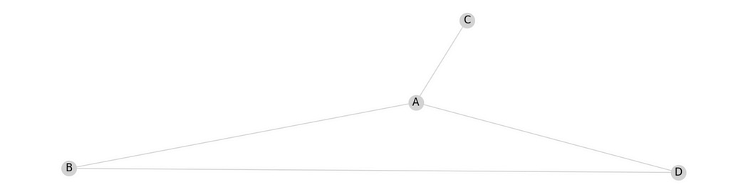

The values of the nodes can be tuples

import networkx as nx
import matplotlib.pyplot as plt

graph = nx.Graph()

graph.add_edge((1,2,3),(1,1,1))
graph.add_edge((1,2,3),(1,1,2))
graph.add_edge((1,2,3),(3,3,3))
graph.add_edge((3,3,3),(1,1,1))

plt.figure(figsize=(12, 3))
nx.draw(graph, with_labels=True, node_color='lightgray', edge_color='lightgray')

They can even be functions

import networkx as nx
import matplotlib.pyplot as plt

def func_a(arg):
    print('a', arg)

def func_b(arg):
    print('b', arg)

def func_c(arg):
    print('c', arg)

def func_d(arg):
    print('d', arg)

import networkx as nx
import matplotlib.pyplot as plt

graph = nx.Graph()

graph.add_edge(func_a,func_b)
graph.add_edge(func_a,func_c)
graph.add_edge(func_a,func_d)
graph.add_edge(func_d,func_b)

plt.figure(figsize=(12, 3))
nx.draw(graph, with_labels=True, node_color='lightgray', edge_color='lightgray')

The only constraint is that the values have to be “hashable”, meaning your programming language can turn the values into a representation such that it can compare two nodes. This is important for ensuring that nodes are a set and that there aren’t duplicates. If you’re curious about how this shakes out, research the hash function in Python.

You might have noticed that each of the graphs we rendered looks slightly different. If we use the nx.draw function to draw the same graph multiple times, we’ll get several different views of the same graph.

import networkx as nx
import matplotlib.pyplot as plt

#creating graph
graph = nx.Graph()

#adding edges
graph.add_edge(1,2)
graph.add_edge(1,3)
graph.add_edge(1,4)
graph.add_edge(4,2)
graph.add_edge(4,5)
graph.add_edge(6,5)
graph.add_edge(6,7)
graph.add_edge(6,8)
graph.add_edge(6,9)
graph.add_edge(3,7)

#rendering same graph three times
for i in range(3):
    plt.figure(figsize=(12, 2))
    plt.title(f'representation {i}')
    nx.draw(graph, with_labels=True, node_color='lightgray', edge_color='lightgray')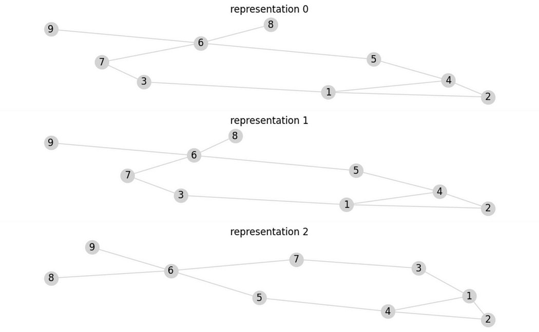

Drawing the smae graph three times yileds three different representations

There is no implicit locational information in a graph, just relative information about which nodes are connected. Thus, there is an infinite number of ways a graph can be rendered.

networkx has a few handy functions that allow you to render the same graph in a variety of ways:

graph = nx.Graph()

graph.add_edge(1,2)
graph.add_edge(1,3)
graph.add_edge(1,4)
graph.add_edge(4,2)
graph.add_edge(4,5)
graph.add_edge(6,5)
graph.add_edge(6,7)
graph.add_edge(6,8)
graph.add_edge(6,9)
graph.add_edge(3,7)

plt.figure(figsize=(12, 3))
plt.title('Spring')
nx.draw_spring(graph, with_labels=True, node_color='lightgray', edge_color='lightgray')

plt.figure(figsize=(12, 3))
plt.title('Planar')
nx.draw_planar(graph, with_labels=True, node_color='lightgray', edge_color='lightgray')

plt.figure(figsize=(12, 3))
plt.title('Circular')
nx.draw_circular(graph, with_labels=True, node_color='lightgray', edge_color='lightgray')

plt.figure(figsize=(12, 3))
plt.title('Spectral')
nx.draw_spectral(graph, with_labels=True, node_color='lightgray', edge_color='lightgray')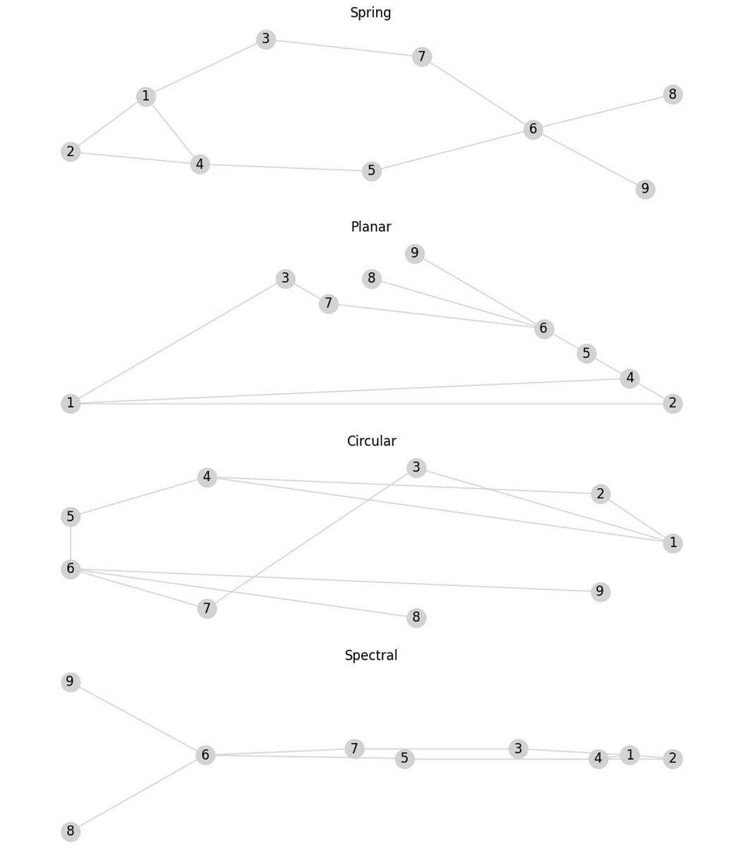

Here:

Spring imagines each edge as a spring that exhibits some force. The nodes are placed randomly, and the springs are allowed to exert their force until the graph reaches an equilibrium.
Planar tries to get all the nodes to be placed such that the edges in the graph do not cross. This isn’t always possible.
Circular arranges all the nodes, sequentially, in a circle.
Spectral uses some fancy math, using something called eigen vectors, to decide on a layout. This example isn’t very good, but this approach can be very helpful when dealing with complex graphs.

Now that we have a handle on some of the basics, let’s dig into the various flavors of graphs.

Types of Graphs

What we’ve been discussing is the “Un-Directed” graph, meaning a graph that describes which nodes are connected but without the concept of directionality. We can also create a “Directed” graph, which does concern direction.

For an un-directed graph, adding the edge (1,2) is equivalent to adding the edge (2,1) . For a directed graph, the edge (1,2) is an edge that points from 1 to 2 , and (2,1) is an edge that points from 2 to 1 . Here, I’m defining the same edges for a directed and un-directed graph.

import networkx as nx
import matplotlib.pyplot as plt

undirected_graph = nx.Graph()

def construct(graph):
    graph.add_edge(1,2)
    graph.add_edge(1,2)
    graph.add_edge(2,1)
    graph.add_edge(1,3)
    graph.add_edge(1,4)
    graph.add_edge(4,2)


#standard, undirected graph
undirected_graph = nx.Graph()
construct(undirected_graph)

#standard, directed graph
directed_graph = nx.DiGraph()
construct(directed_graph)

#rendering both
plt.figure(figsize=(12, 3))
plt.title('Un-Directed')
nx.draw_planar(undirected_graph, with_labels=True, node_color='lightgray', edge_color='gray')
plt.figure(figsize=(12, 3))
plt.title('Directed')
nx.draw_planar(directed_graph, with_labels=True, node_color='lightgray', edge_color='gray', arrows=True)

when defining an un-directed graph, defining the edges (1,2) and (2,1) is redundant, but in the directed graph, it results in nodes 2 and 1 pointing towards each other.

You might notice, in the code above, that the construct function creates the edge (1,2) twice. This is redundant in both the un-directed graph and the directed graph. There’s another type of graph, called a “Multigraph” which does allow for duplicate edges. Multigraphs can either be directed or un-directed, just like normal graphs.

Here, I’m doing some black magic to render the edges so they’re visible, but you don’t have to worry a ton about it. The important part is to understand that a multigraph can have multiple edges between two nodes.

def draw_multigraph(G):
    pos = nx.shell_layout(G)
    nx.draw(G, pos, with_labels=True, node_color='lightgray', edge_color='white', arrows=True)
    for (u, v, k) in G.edges(keys=True):
        nx.draw_networkx_edges(G, pos, edgelist=[(u, v)], connectionstyle=f'arc3,rad={(k - len(G[u][v]) / 2) * 0.2}', edge_color='gray', arrows=True)
    plt.show()

def construct(graph):
    graph.add_edge(1,2)
    graph.add_edge(1,2)
    graph.add_edge(2,1)
    graph.add_edge(1,3)
    graph.add_edge(1,4)
    graph.add_edge(4,2)

#multi undirected graph
multi_graph = nx.MultiGraph()
construct(multi_graph)

multi_directed_graph = nx.MultiDiGraph()
construct(multi_directed_graph)

plt.figure(figsize=(12, 3))
plt.title('Un-Directed Multigraph')
draw_multigraph(multi_graph)

plt.figure(figsize=(12, 3))
plt.title('Directed Multigraph')
draw_multigraph(multi_directed_graph)

MultiGraphs certainly have their place, but most problems can be expressed more elegantly with traditional graphs, so we won’t be using them throughout this article.

Let’s explore a few ways of defining graphs next. This will be handy as it will allow us to create some complex graphs, which will help as we explore graph analysis.

Methods of Defining Graphs

Previously, we used the add_edge function to add edges one by one. This is perfectly fine, but there are a variety of other approaches for defining graphs that may be useful in different use cases. Here are a few ways of defining the same graph:

import numpy as np

#adding edges one by one
graph1 = nx.Graph()
graph1.add_edge(1, 2)
graph1.add_edge(2, 3)
graph1.add_edge(3, 1)

#adding list of edges
graph2 = nx.Graph()
graph2.add_edges_from([(1, 2), (2, 3), (3, 1)])

#defining a graph based on a list of edges
edges = [(1, 2), (2, 3), (3, 1)]
graph3 = nx.from_edgelist(edges)

#this can be also be done by passing the edge list in the Graph constructor
graph5 = nx.Graph([(1, 2), (2, 3), (3, 1)])

#using an adjacency dictionary (which nodes are connected with which other nodes)
adj_dict = {1: [2, 3], 2: [1, 3], 3: [1, 2]}
graph6 = nx.Graph(adj_dict)

#using an adjacency matrix
adj_matrix = np.array([
    [0, 1, 1],
    [1, 0, 1],
    [1, 1, 0]
])
graph7 = nx.from_numpy_array(adj_matrix)

Most of these are pretty straightforward, except perhaps the idea of “an adjacency matrix”. In an adjacency matrix, there’s a spot for each possible connection; then you place a 1 if there is a connection, and a 0 if there isn’t a connection.

the adjacency matrix specifies which nodes are connected with which other nodes. This particular matrix specifies that each node is connected with each other node, and that the nodes do not have edges which connect a node with themselves. Depending on how this matrix is filled out, you can also specify directionality in this matrix, where rows are the node which an edge is coming from, and columns are the node which the edge is pointing towards.

When defining a graph based on an adjacency matrix, there are no labels, so graph7 is slightly different from the other graphs in this example. It should still have the same structure, though, which we can test with nx.is_isomorphic (isomorphism being two graphs having the same structure)

"""Checking if all the graphs have the same structure
"""

import networkx as nx

graphs = [graph1, graph2, graph3, graph4, graph5, graph6]
n = len(graphs)

# Compare every graph with every other graph
isomorphic_groups = []
checked = set()

for i in range(n):
    for j in range(i + 1, n):
        if (i, j) not in checked:
            if nx.is_isomorphic(graphs[i], graphs[j]):
                isomorphic_groups.append((f"G{i+1}", f"G{j+1}"))
            else:
                raise ValueError('Not Isomorphic!')
            checked.add((i, j))

print('all graphs isomorphic (the same)')

Another useful way of defining a graph is by defining a “complete graph”. A complete graph is what you get when you fully connect some number of nodes. This is usually denoted as k{n} where n is the number of nodes. For instance, we can define a k4 graph with the following code:

"""Defining a complete graph
"""

graph = nx.complete_graph(4)
plt.figure(figsize=(12, 3))
nx.draw_circular(graph, with_labels=True, arrows=True, node_color='lightgray', edge_color='gray')
plt.show()

Naturally, this can be done with an arbitrary number of nodes. Here, I’m defining a k4 , k5 , k6 , and k7 graph.

"""Defining a few complete graphs of various sizes
"""

import networkx as nx
import matplotlib.pyplot as plt

fig, axes = plt.subplots(2, 2, figsize=(12, 8))  # 2x2 layout

sizes = [4, 5, 6, 7]  # Different complete graph sizes

for ax, n in zip(axes.flatten(), sizes):
    G = nx.complete_graph(n)
    pos = nx.circular_layout(G)  # Use circular layout
    nx.draw(G, pos, with_labels=True, arrows=True, node_color='lightgray', edge_color='gray', ax=ax)
    ax.set_title(f'K{n}')  # Title for each graph

plt.tight_layout()
plt.show()

Ok, cool, we’ve created a few graphs. Let’s go over some basic manipulation in the next section, then, we’ll explore more advanced graph manipulation and processing in the following sections.

Basic Graph Manipulation

One very useful operation when working with graphs is extracting a sub-graph. This extracts some subset of nodes from all of the nodes in the graph and also extracts all of the edges between those nodes.

"""extracting a subgraph from a K7 complete graph
"""

import networkx as nx

G = nx.complete_graph(7)
subgraph = G.subgraph([2,3,4,6])
nx.draw_circular(subgraph, with_labels=True, arrows=True, node_color='lightgray', edge_color='gray')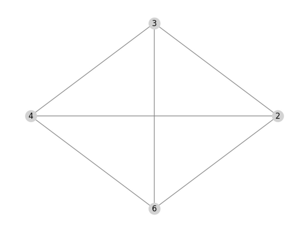

the subgraph of nodes 2,3,4, and 6 from a k7 graph.

We can also connect graphs.

Here, I’m defining a k4 graph (so, nodes {0,1,2,3}) and a k3 graph (nodes {0,1,2}) and then I’m re-naming the nodes in the k3 graph to {4,5,6}, which is necessary because when you combine two graphs, it will merge nodes with the same value. We can also define a third graph, with nodes {0,4} and a connection between them. If we combine all three of those graphs, we’ll get the following:

"""creating three graphs and connecting them together
"""

import networkx as nx
import matplotlib.pyplot as plt

# Create two separate graphs
G1 = nx.complete_graph(4)  # First complete graph K4
G2 = nx.complete_graph(3)  # Second complete graph K3
nx.relabel_nodes(G2, {i: i + 4 for i in G2.nodes()}, copy=False)  # Shift node labels

# Merge the two graphs by adding a bridge edge
G_combined = nx.compose(G1, G2)
G_combined.add_edge(0, 4)  # Connect Graph 1 to Graph 2

# Function to plot a graph
def plot_graph(G, title, pos=None):
    if pos is None:
        pos = nx.spring_layout(G, seed=42)
    plt.figure(figsize=(12, 4))
    nx.draw(G, pos, with_labels=True, node_color='lightgray', edge_color='gray', arrows=True)
    plt.title(title)
    plt.show()
    return pos

# Plot the combined graph
pos = plot_graph(G_combined, "Combined Graph (K4 + K3)")

If we remove the edge (0,4) from this graph, we’ll get a single graph with two “islands”, islands being isolated components of the graph that share no connections.

# Remove the connecting edge
G_combined.remove_edge(0, 4)
plot_graph(G_combined, 'combined graph with (0,4) removed')
plt.show()

We can use the connected_components function to get the list of components for each island and use the subgraph function to extract those components into separate subgraphs.

# Detect connected components (islands)
subgraphs = [G_combined.subgraph(c).copy() for c in nx.connected_components(G_combined)]

# Step 3: Plot each separated component
for i, subG in enumerate(subgraphs):
    plot_graph(subG, f"Separated Graph {i+1}", pos)

Combining, separating, and renaming graphs is fundamental in most practical applications of graphs as it allows for granular analysis and exploration.

Now that we’re getting more familiar with graphs, I think it might be useful to cover a few important metrics that data scientists use to describe graphs.

Key Graph Metrics

If you want to count the number of connections a particular node has, we call that the “degree”

"""For an un-directed graph, the degree of a node is the number of connections
"""

graph = nx.Graph([(1, 2), (2, 3), (3, 1), (4, 1), (1, 3)])
nx.draw_circular(graph, with_labels=True, arrows=True, node_color='lightgray', edge_color='gray')
plt.plot()
print('degree of each node: ', graph.degree)

The degree of each node. node 1 is degree 3, because it has three connections. Node 2 is degree 2, because it has two connections. Etc.

The degree of a node becomes a bit more complex when we consider directed graphs. In directed graphs, the “in degree” is the number of connections going into the node, the “out degree” is the number of connections going out of the node, and the “degree” is the sum of the in and out degrees.

""" for a directed graph, the degree is the number of outgoing and ingoing conenctions
degree = in_degree + out_degree
"""

edges = [(0, 0), (1, 0), (1, 2), (2, 0), (2, 1), (2, 3), (3, 2)]
graph = nx.DiGraph(edges)

print('degree:     ', dict(graph.degree))
print('in degree:  ', dict(graph.in_degree))
print('out degree: ', dict(graph.out_degree))

nx.draw_circular(graph, with_labels=True, arrows=True, node_color='lightgray', edge_color='gray')

Depending on the context in which a graph is being applied, the degree might correspond to the number of friends someone has, the number of transactions an entity makes, whatever.

Another super useful metric is the shortest path between two nodes, which can be calculated with nx.shortest_path . That takes in a graph, start, and end node and spits out a list of nodes.

"""Creating a graph and finding the shortest path between nodes 1 and 5
"""

# Create a sample graph
G = nx.Graph([(1, 2), (2, 3), (3, 4), (4, 5), (2, 6), (6, 7), (7, 8), (8,5)])

# Draw nodes
nx.draw(G, pos, with_labels=True, node_color="lightgray", edge_color="gray", node_size=800, font_size=12)

shortest_path = nx.shortest_path(G, source=1, target=5)
print(f"Shortest path from 1 to 5: {shortest_path}")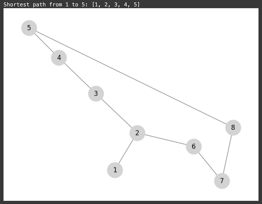

“Radius” and “eccentricity” are other key metrics, which are built on top of the shortest distance. The “eccentricity” of a node is the longest shortest path that node has to any other node. You might imagine that nodes on the outer borders of a graph might have a very long shortest path to nodes on the other side of the graph, while nodes in the middle might have a relatively short shortest path to all other nodes. Thus, the “eccentricity” is a measure of how eccentric (on the edge) a particular node is.

The “Radius” of a graph is the smallest eccentricity, which can be thought of as how wide a graph is from the center.

The following code calculates the radius og a graph and the eccentricity of all nodes in that graph and highlights the nodes whose eccentricity is equal to the radius. These nodes are “central”, meaning they’re in the middle of the graph.

"""calculating the eccentricity (longest shortest path) for each node
and the radius (shortest eccentricity of all nodes) of the graph
"""

import networkx as nx
import matplotlib.pyplot as plt

# Create a sample graph
G = nx.Graph([(1, 2), (2, 3), (3, 4), (4, 5), (2, 6), (6, 7), (6, 8)])

# Compute eccentricities (greatest shortest path)
eccentricities = nx.eccentricity(G)
print('eccentricities: ', eccentricities)

# Compute radius (minimum eccentricity)
radius = nx.radius(G)

# Find the central node(s) (nodes with eccentricity equal to the radius)
central_nodes = [node for node, ecc in eccentricities.items() if ecc == radius]

# Draw the graph
pos = nx.spring_layout(G)
plt.figure(figsize=(6, 4))

# Draw nodes
nx.draw(G, pos, with_labels=True, node_color="lightgray", edge_color="gray", node_size=800, font_size=12)

# Highlight central nodes
nx.draw_networkx_nodes(G, pos, nodelist=central_nodes, node_color="red", node_size=800)

# Show the radius
plt.title(f"Graph Radius: {radius} (Red nodes are central)")
plt.show()

the eccentricities of all nodes, with the central nodes highlighted in red. The radius of this graph is 3.

Here, we defined centrality based on eccentricity, but there are other ways to define which nodes are central, which may be useful in other applications.

Centrality

The idea of “centrality” can be a bit philosophical when it comes to graphs. Are central nodes well-connected nodes? Are they the nodes through which the shortest paths pass? Are they the nodes with the lowest eccentricity, like in the previous section? The answer really depends on what you care about, which is why there are a few ways of calculating centrality within a graph.

Here, I’m calculating a few different approaches:

degree_centrality = nx.degree_centrality(graph)
betweenness_centrality = nx.betweenness_centrality(graph)
closeness_centrality = nx.closeness_centrality(graph)
eigenvector_centrality = nx.eigenvector_centrality(graph)

# Plot Centrality Measures
fig, axs = plt.subplots(2, 2, figsize=(12, 10))
centralities = {
    'Degree Centrality': degree_centrality,
    'Betweenness Centrality': betweenness_centrality,
    'Closeness Centrality': closeness_centrality,
    'Eigenvector Centrality': eigenvector_centrality
}

pos = nx.spring_layout(graph, seed=42)

for ax, (title, centrality) in zip(axs.flatten(), centralities.items()):
    node_sizes = [v * 2000 for v in centrality.values()]
    nx.draw(graph, pos, with_labels=True, node_size=node_sizes, edge_color='gray', ax=ax)
    ax.set_title(title)

plt.show()

Here,

Degree Centrality is judging centrality by how many connections a node has. By this definition, the node labeled “middle” is the least central, as it has the fewest number of connections.
Betweenness Centrality is judging centrality by how many shortest paths go through a node. Here, many shortest paths go through the node labeled “middle”, so it scores high on this metric of centrality.
Closeness Centrality is judging based on the average distance to all other nodes. It seems like, by this metric, the node labeled “middle” might be marginally more central, but not much.
Eigenvector Centrality is a bit complex mathematically, but the essential idea is that it accounts for how impactful the neighbors of a particular node are. So, a node may be deemed “central” based on how important neighboring nodes are, even if it would rank low on all other metrics of centrality.

Cliques

I was watching a video on graphs by someone who didn’t speak English as a native language. If that’s you, the intuition of a “clique” might be lost.

The word “Clique” is used in both American and British English to describe a tight, exclusive group of friends within a larger network of friends. A “Clique” in graph theory is a complete sub-graph within a larger graph. We can find cliques with the following code:

#find maximal complete subgraphs
print(list(nx.find_cliques(graph)))
nx.draw_spring(graph, with_labels=True)

A graph, and the cliques within that graph

We can filter by graphs of a certain size by using the k_core function, which finds all of the islands that are a fully connected graph of some size

# Compute the k-core subgraph (nodes with degree >= 5)
well_connected_islands = nx.k_core(graph, k=5)

# Define positions for consistent layout
pos = nx.spring_layout(graph)

# Plot both graphs side by side
fig, axes = plt.subplots(1, 2, figsize=(12, 6))

# Plot original graph
axes[0].set_title("Original Graph")
nx.draw(graph, pos, ax=axes[0], with_labels=True, node_color="lightblue", edge_color="gray", node_size=800)

# Plot k-core subgraph
axes[1].set_title("Well-Connected Islands (k=5)")
nx.draw(well_connected_islands, pos, ax=axes[1], with_labels=True, node_color="red", edge_color="black", node_size=800)

# Show the plots
plt.show()

nx.kcore creates a graph called well_connected_islands based on preserving islands that are equivalent to a k5 fully connected graph or higher. well_connected_islands is perhaps a bit of a misnomer because it’s a single graph that contains all the islands. We could use nx.connected_components to identify the islands in this graph to actually list out the islands within the well_connected_islands graph.

"""finding the islands in the well_connected_islands graph.
"""

nx.draw(well_connected_islands, pos, with_labels=True)
print(list(nx.connected_components(well_connected_islands)))

Cliques are a useful general idea because they allow one to isolate very tightly grouped regions within a larger graph. The following section defines a few more structures that can also be useful in understanding the structure of a graph.

Have any questions about this article? Join the IAEE Discord.

Join The Discord

Bridges, Local Bridges, and Connection Strength

A bridge is an edge that is responsible for connecting two portions of a graph together, such that if the bridge were removed, you would create an island.

"""Finding bridges
edges which, if they were removed, would create isolated subgraphs
"""

graph1 = nx.complete_graph(6)
graph2 = nx.complete_graph(6)
graph2 = nx.relabel_nodes(graph2, {0: 'A', 1: 'B', 2: 'C', 3: 'D', 4: 'E', 5: 'F'})
connection = nx.from_edgelist([(0, 'middle'), (1, 'middle'), ('middle', 'A')])
graph = nx.compose_all([graph1, graph2, connection])
nx.draw_spring(graph, with_labels=True)

#finding and printing out all bridges
print(list(nx.bridges(graph)))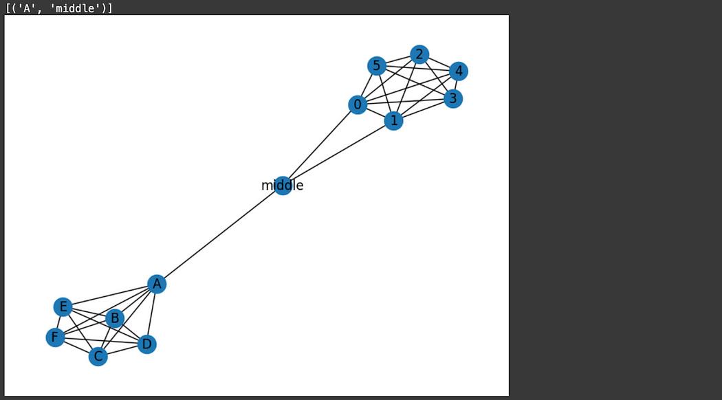

This is useful, especially in simple graphs, however, complex graphs with many connections might have very few bridges as, technically, there is some other roundabout way that connects two regions of the graph together.

A “Local Bridge” is a bridge that would not create two sub-graphs if removed, but removing that connection would make it take longer to traverse between two nodes. Take the following code, for example, which defines a graph and calculates the local bridges:

"""Finding bridges
edges which, if they were removed, would create isolated subgraphs
"""

graph1 = nx.complete_graph(6)
graph2 = nx.complete_graph(6)
graph2 = nx.relabel_nodes(graph2, {0: 'A', 1: 'B', 2: 'C', 3: 'D', 4: 'E', 5: 'F'})
connection = nx.from_edgelist([(0, 'middle'), (1, 'middle'), ('middle', 'A'), (2, 'E')])
graph = nx.compose_all([graph1, graph2, connection])
nx.draw_spring(graph, with_labels=True)

#find and print out local bridges
print(list(nx.local_bridges(graph)))

Here, the function local_bridges returns [(2, ‘E’, 4), (‘A’, ‘middle’, 4)] where:

(2, ‘E’, 4) means that removing the edge between 2 and E would mean you need to take 4 steps to navigate to navigate from 2 to E
(‘A’, ‘middle’, 4) means that removing the edge between A and middle would mean you need to take 4 steps to navigate from A to middle

You might be able to imagine that different local bridges might have different amounts of importance, as some might cause only slight increases in distance between nodes if removed, and some might cause large increases in distance between nodes if removed.

In directed graphs, the concept of a bridge still holds, but as there is direction, there is a more nuanced interpretation of what a “connection” really means.

Take the following graph:

import networkx as nx
import matplotlib.pyplot as plt

# Create a directed graph
G = nx.DiGraph()

# Add edges (arrows)
G.add_edges_from([(1, 2), (2, 3), (3, 1),  # A cycle (strongly connected)
                  (4, 5), (5, 6), (6, 4),  # Another cycle (strongly connected)
                  (3, 4), (6, 7)])         # One-way connections

# Draw the original graph
plt.figure(figsize=(10, 5))
pos = nx.spring_layout(G)

Each of these nodes is connected, but some of them can be thought of as “more” connected. For instance, nodes 4 , 5 , and 6 can each visit each other regardless of the starting point, whereas nodes 3 and 4 are less strongly connected as node 3 points to node 4 , but there’s no way to traverse from node 4 to node 3 .

This idea is formalized as “strongly” and “weakly” connected components. A strongly connected component is a subgraph where all nodes can be navigated to from all other nodes. Weakly connected components are subgraphs where all nodes can be visited, but you might not be able to visit every node from every other node.

In this example, all the nodes are weakly connected, but there are sub-graphs that are strongly connected.

import networkx as nx
import matplotlib.pyplot as plt

# Create a directed graph
G = nx.DiGraph()

# Add edges (arrows)
G.add_edges_from([(1, 2), (2, 3), (3, 1),  # A cycle (strongly connected)
                  (4, 5), (5, 6), (6, 4),  # Another cycle (strongly connected)
                  (3, 4), (6, 7)])         # One-way connections

# Find groups of strongly and weakly connected nodes
sccs = list(nx.strongly_connected_components(G))
wccs = list(nx.weakly_connected_components(G))

# Draw the original graph
plt.figure(figsize=(10, 5))
pos = nx.spring_layout(G)

# Draw all nodes and arrows
nx.draw(G, pos, with_labels=True, node_size=800, edge_color="gray", node_color="lightblue", arrows=True)

# Print out the connected groups
print("Strongly Connected Components:", sccs)
print("Weakly Connected Components:", wccs)

plt.title("Strongly and weakly connected components")
plt.show()

Eulerian Paths

In graph theory, an “Eulerian Path” is one in which, if you traversed through a graph edge-by-edge, you would traverse through all edges on the graph exactly once. Imagine you were a janitor sweeping the floors in a large building, and you want to walk through each hallway once and not have to backtrack or pass through a hallway you’ve already been through before.

Not all graphs have eulerian paths, but you can use the has_eulerian_path function to evaluate if a graph has an eulerian path, and the eulerian_path function to actually get the path.

import networkx as nx
import matplotlib.pyplot as plt

# Create a graph with an Eulerian path
G = nx.Graph()
edges = [(0, 1), (1, 2), (2, 3), (3, 0), (0, 4), (4, 2)]
G.add_edges_from(edges)

# Check if the graph has an Eulerian path
has_eulerian_path = nx.has_eulerian_path(G)

# Find and print the Eulerian path if it exists
if has_eulerian_path:
    eulerian_path = list(nx.eulerian_path(G))
    print("Eulerian Path:", eulerian_path)
else:
    print("No Eulerian Path exists in this graph.")

# Draw the graph
plt.figure(figsize=(6, 4))
pos = nx.spring_layout(G)
nx.draw(G, pos, with_labels=True, node_size=800, edge_color="gray", node_color="lightblue")
plt.title("Graph with Eulerian Path" if has_eulerian_path else "No Eulerian Path Exists")
plt.show()

Weighted Graphs

A common embellishment to the traditional graph is the “weighted” graph, where each edge is assigned some weight.

import networkx as nx
import matplotlib.pyplot as plt

# Create a graph
G = nx.Graph()

# Add weighted edges (node1, node2, weight)
edges = [(0, 1, 2.5), (1, 2, 1.2), (2, 3, 3.8), (3, 4, 2.1), (4, 0, 4.0), (1, 4, 2.7)]
G.add_weighted_edges_from(edges)

# Define node positions
pos = nx.spring_layout(G)

# Draw the graph
plt.figure(figsize=(6, 4))
nx.draw(G, pos, with_labels=True, node_size=800, edge_color="gray", node_color="lightblue")

# Draw edge labels (weights)
edge_labels = {(u, v): w for u, v, w in edges}
nx.draw_networkx_edge_labels(G, pos, edge_labels=edge_labels, font_size=12)

# Show the graph
plt.title("Weighted Graph Example")
plt.show()

This has a wide range of practical uses. It can be used for GPS routing based on traffic patterns, be used to describe how closely two entities are related, and serves as the fundamental conceptualization of neural networks, the bedrock of modern AI.

Neural Networks — Intuitively and Exhaustively Explained

Daniel Warfield

Jan 30

Read full story

The shortest path can be found in a weighted graph using the nx.shortest_path function with the weight=’weight’ argument. The longest path is a bit tricker to compute because most people don’t care about it, but we can calculate it by iterating over all paths between two nodes and simply finding the path with the maximum value.

import networkx as nx
import matplotlib.pyplot as plt
from matplotlib.lines import Line2D  # Import for custom legend

# Create a weighted graph
G = nx.Graph()

# Add weighted edges (node1, node2, weight)
edges = [(0, 1, 2.5), (1, 2, 1.2), (2, 3, 3.8), (3, 4, 2.1), (4, 0, 4.0), (1, 4, 2.7)]
G.add_weighted_edges_from(edges)

# Find the **shortest path (minimum weight)**
min_path = nx.shortest_path(G, source=0, target=2, weight='weight')
min_weight = nx.shortest_path_length(G, source=0, target=2, weight='weight')

# Find the **longest path (maximum weight)**
all_paths = list(nx.all_simple_paths(G, source=0, target=2))  # Get all paths from 0 to 2
max_path = max(all_paths, key=lambda path: sum(G[u][v]['weight'] for u, v in zip(path, path[1:])))
max_weight = sum(G[u][v]['weight'] for u, v in zip(max_path, max_path[1:]))

# Draw the graph
plt.figure(figsize=(6, 4))
pos = nx.spring_layout(G)

# Draw all nodes and edges
nx.draw(G, pos, with_labels=True, node_size=800, edge_color="gray", node_color="lightblue")

# Draw edge labels (weights)
edge_labels = {(u, v): w for u, v, w in edges}
nx.draw_networkx_edge_labels(G, pos, edge_labels=edge_labels, font_size=12)

# Highlight the minimum-weight path in **green**
nx.draw_networkx_edges(G, pos, edgelist=list(zip(min_path, min_path[1:])), edge_color="green", width=2.5)

# Highlight the maximum-weight path in **red**
nx.draw_networkx_edges(G, pos, edgelist=list(zip(max_path, max_path[1:])), edge_color="red", width=2.5, style="dashed")

# Create a fixed legend using Line2D
legend_elements = [
    Line2D([0], [0], color="green", lw=2.5, label="Min Weight Path"),
    Line2D([0], [0], color="red", lw=2.5, linestyle="dashed", label="Max Weight Path"),
]

# Add the legend
plt.legend(handles=legend_elements, loc="upper right")

plt.title("Weighted Graph with Min & Max Paths")
plt.show()

# Print the Eulerian Path
print(f"Minimum weight path from 0 to 2: {min_path} (Weight: {min_weight})")
print(f"Maximum weight path from 0 to 2: {max_path} (Weight: {max_weight})")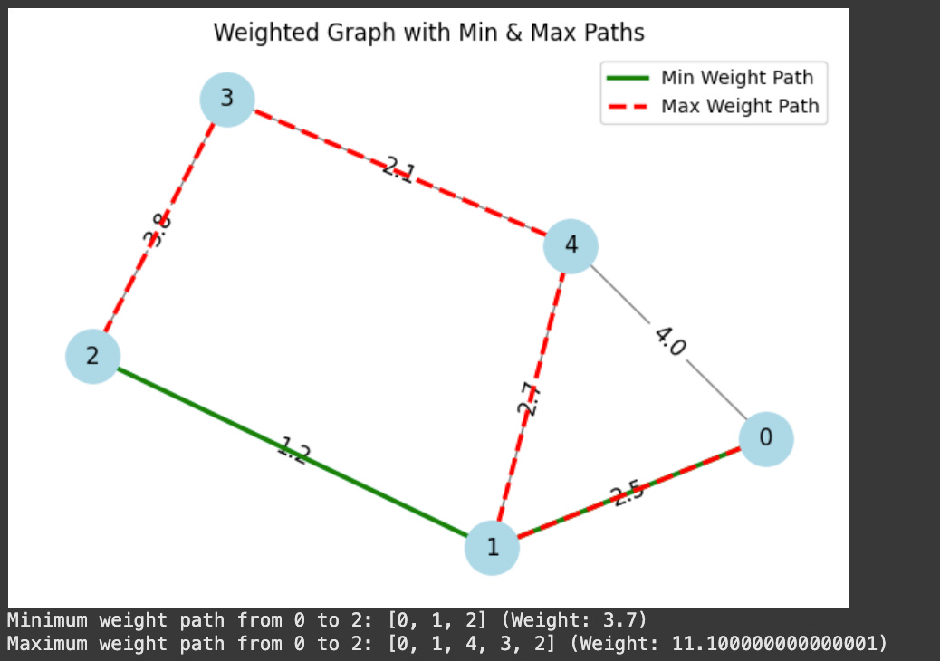

Graph Coloring

Graph Coloring is a subtly complex idea within graph theory that concerns how one might choose to label connected nodes within a graph.

Imagine you want to choose a color for all the nodes in a graph, such that no two connected nodes would have the same color. The question of graph coloring is, first, how many colors do you need and, two, what does each node get colored.

Thankfully, you can avoid a week of math classes and just use nx.coloring to find this stuff out for you.

import networkx as nx
import matplotlib.pyplot as plt

# Create a simple graph
G = nx.Graph()
edges = [(0, 1), (0, 2), (1, 2), (1, 3), (2, 3), (3, 4), (4, 5), (5, 0)]
G.add_edges_from(edges)

# Use a greedy algorithm to color the graph
coloring = nx.coloring.greedy_color(G, strategy="largest_first")  # Assigns colors

# Get unique colors
num_colors = len(set(coloring.values()))

# Define colors for visualization
node_colors = [coloring[node] for node in G.nodes]

# Draw the graph
plt.figure(figsize=(6, 4))
pos = nx.spring_layout(G)
nx.draw(G, pos, with_labels=True, node_size=800, node_color=node_colors, cmap=plt.cm.rainbow, edge_color="gray")

# Show results
plt.title(f"Graph Coloring Example (Chromatic Number = {num_colors})")
plt.show()

print("Node Coloring:", coloring)
print(f"Chromatic Number: {num_colors}")

Don’t ask me to prove it, but there’s a fun idea in graph theory called the “four color theorem” which states that any planar graph (a graph that can be drawn in 2D with no overlapping edges) can be colored with a maximum of four colors. If you’ve ever taken a mapping class and you had to color adjacent countries with different colored pencils, you might know you only ever need a maximum of four colors. That’s why!

There’s some other theory I’m not covering in this article, feel free to check out the code for a few more interesting ideas like Hamiltonian paths. For now, though, let’s dive into some practical examples!

Practical Applications

Practical Application 1) Traveling Salesman

It wouldn’t be a discussion about graphs without the traveling salesman.

In the traveling salesman problem, one imagines oneself as a salesman who is tasked with traversing from town to town. Each of these towns has some distance between them, and the objective is to travel to each town while minimizing the total distance traveled.

Here, the function nx.approximation.traveling_salesman_problem can be used to approximate the shortest path. It expects an argument for the graph, whether or not the salesman has to travel in a cycle or just has to visit every node once, and the weight. The rest of the code is just for rendering.

import networkx as nx
import matplotlib.pyplot as plt

# Create a more complex weighted graph
G = nx.Graph()

# Define a larger set of edges with weights (distances or costs)
edges = [
    (0, 1, 10), (0, 2, 15), (0, 3, 20), (0, 4, 25),
    (1, 2, 35), (1, 3, 25), (1, 4, 30), (1, 5, 20),
    (2, 3, 30), (2, 4, 20), (2, 5, 25), (2, 6, 15),
    (3, 4, 10), (3, 5, 30), (3, 6, 20), (3, 7, 25),
    (4, 5, 15), (4, 6, 35), (4, 7, 20), (5, 6, 10),
    (5, 7, 15), (6, 7, 10)
]

# Add the weighted edges to the graph
G.add_weighted_edges_from(edges)

# Use an approximation algorithm to find a good solution for the Traveling Salesman Problem
best_route = nx.approximation.traveling_salesman_problem(G, cycle=True, weight='weight')

# Calculate the total travel cost (sum of all edge weights in the route)
total_weight = sum(G[u][v]['weight'] for u, v in zip(best_route, best_route[1:]))

# Draw the graph
plt.figure(figsize=(8, 6))  # Set a larger figure size for better visualization
position = nx.spring_layout(G, seed=42)  # Use a fixed seed for consistent positioning

# Draw all nodes and edges in the graph
nx.draw(G, position, with_labels=True, node_size=800, node_color="lightblue", edge_color="gray")

# Label the edges with their respective weights (distances)
edge_labels = {(u, v): w for u, v, w in edges}
nx.draw_networkx_edge_labels(G, position, edge_labels=edge_labels, font_size=10)

# Highlight the found Traveling Salesman route in red
route_edges = list(zip(best_route, best_route[1:]))  # Convert the path into a list of edges
nx.draw_networkx_edges(G, position, edgelist=route_edges, edge_color="red", width=2.5)

# Display the graph
plt.title(f"Best Found Route for Traveling Salesman Problem (Total Distance: {total_weight})")
plt.show()

# Print the best-found route and its total travel cost
print("Best Found Route:", best_route)
print("Total Distance (Travel Cost):", total_weight)

Obviously this isn’t only useful for salesman. Finding the shortest path through all nodes in a graph is useful for optimizing delivery routes, manufacturing processes, and even pops in in sequencing DNA.

Practical Application 2) Scheduling

Let’s imagine ourselves as faculty members in a university, with summer rapidly approaching and final exams upon us. In this scenario, we might find ourselves met with a dilemma: We have many students who take multiple classes, but the more final exam time slots we need to host, the less piña colada we can consume. Wouldn’t it be nice if we could find the fewest exam slots necessary so that each student can take an exam without conflict?

We previously discussed graph coloring, which is the general problem of finding colors for each node in a graph where no connected nodes have the same color. If we construct a graph where nodes represent classes and edges represent if there is a student taking both of those classes this semester, we can use graph coloring to help us find how many exam slots we need and which classes should occupy which slots.

Here, the lion's share of the work is done with nx.coloring.greedy_color , with the rest of the code chiefly going into rendering.

import networkx as nx
import matplotlib.pyplot as plt

# Create a more complex exam scheduling graph
G = nx.Graph()

# Define a larger set of courses and their conflicts (shared students)
edges = [
    ("Math", "Physics"), ("Math", "Chemistry"), ("Math", "Computer Science"),
    ("Physics", "Biology"), ("Physics", "English"), ("Physics", "Computer Science"),
    ("Chemistry", "Biology"), ("Chemistry", "History"), ("Chemistry", "Economics"),
    ("Biology", "History"), ("Biology", "Economics"), ("Biology", "Computer Science"),
    ("English", "History"), ("English", "Economics"), ("English", "Political Science"),
    ("History", "Political Science"), ("History", "Geography"), ("Economics", "Political Science"),
    ("Economics", "Geography"), ("Computer Science", "Political Science"), ("Geography", "Physics"),
    ("Political Science", "Math"), ("Political Science", "Computer Science")
]

# Add edges to the graph
G.add_edges_from(edges)

# Apply graph coloring to schedule exams
exam_schedule = nx.coloring.greedy_color(G, strategy="largest_first")

# Get the number of unique time slots required
num_timeslots = len(set(exam_schedule.values()))

# Assign colors for visualization
node_colors = [exam_schedule[node] for node in G.nodes]

# Draw the graph
plt.figure(figsize=(10, 6))
pos = nx.spring_layout(G, seed=42)  # Seed for consistent layout
nx.draw(G, pos, with_labels=True, node_size=1200, node_color=node_colors, cmap=plt.cm.rainbow, edge_color="gray", font_size=10)

# Show results
plt.title(f"Complex Exam Scheduling Graph (Time Slots Needed = {num_timeslots})")
plt.show()

# Print the exam schedule
print("Exam Schedule (Course -> Time Slot):")
for course, slot in sorted(exam_schedule.items(), key=lambda x: x[1]):
    print(f"{course}: Time Slot {slot}")

Practical Application 3) Page Rank

If you’re a company like Google, you have a vested interest in knowing which websites are more popular/important. One way Google does this is with an algorithm called “PageRank” which, in essence, ranks certain websites based on which websites link to that website and how important those websites are. This is a fascinating topic that is worthy of a deep dive within itself (it employs an idea of a random surfer and attempts to calculate their probability of landing on a particular page), but luckily for us networkx has an implementation of pagerank which we can just use.

import networkx as nx
import matplotlib.pyplot as plt

# Create a directed network of links
G = nx.DiGraph()
edges = [("ZetaHub.net", "AlphaSphere.io"), ("ZetaHub.net", "QuantumFlux.org"), 
         ("AlphaSphere.io", "NeonVista.biz"), ("QuantumFlux.org", "NeonVista.biz"), 
         ("NeonVista.biz", "ZetaHub.net"), ("EchoBridge.ai", "ZetaHub.net"), 
         ("EchoBridge.ai", "QuantumFlux.org"), ("EchoBridge.ai", "NeonVista.biz")]

G.add_edges_from(edges)

G.add_edges_from(edges)

# Compute PageRank
pagerank_scores = nx.pagerank(G)

# Draw the network, scaling node size by PageRank score
plt.figure(figsize=(6, 4))
pos = nx.spring_layout(G)
node_sizes = [10000 * pagerank_scores[node] for node in G.nodes]

nx.draw(G, pos, with_labels=True, node_size=node_sizes, node_color="lightblue", edge_color="gray", arrows=True)
plt.title("PageRank in a Network of Links")
plt.show()

# Print PageRank scores
print("PageRank Scores:")
for user, score in sorted(pagerank_scores.items(), key=lambda x: x[1], reverse=True):
    print(f"{user}: {score:.4f}")

In this particular example, the node “NeonVista.biz” is deemed high rank because two fairly high ranking nodes connect to it, and “ZetaHub.net” is high rank because a very high ranking node points to it.

This can be used for a variety of applications. For instance, choosing which order to rank search results on a website like Google.

Practical Applications 4) Influence Maximization

Let’s say you worked at a media company and wanted to kick off an ad campaign to market a certain product. You had a selection of social media users, and you wanted to identify which ones you wanted to approach for a paid partnership. The hope would be that there might be some network effect where the content made from your paid users sparks some conversation about the product as their followers talk to their followers.

In this case, using “centrality” might be useful. The more central a node is, the more closely connected that node is to other nodes.

import networkx as nx
import matplotlib.pyplot as plt

# Using a pre-made graph from nx, based on charecter relations in les mis
G = nx.les_miserables_graph()

# Compute different types of centrality
degree_centrality = nx.degree_centrality(G)
betweenness_centrality = nx.betweenness_centrality(G)
closeness_centrality = nx.closeness_centrality(G)

# Function to find the top n nodes for a given centrality measure
def top_nodes(centrality_dict, num=5):
    return sorted(centrality_dict, key=centrality_dict.get, reverse=True)[:num]

top_degree = top_nodes(degree_centrality)
top_betweenness = top_nodes(betweenness_centrality)
top_closeness = top_nodes(closeness_centrality)

# Layout for the graph
pos = nx.spring_layout(G)

# Create subplots
fig, axes = plt.subplots(1, 3, figsize=(15, 5))

# Plot for Degree Centrality
axes[0].set_title("Degree Centrality")
nx.draw(G, pos, ax=axes[0], with_labels=True, node_color="lightblue", edge_color="gray", node_size=600)
nx.draw_networkx_nodes(G, pos, ax=axes[0], nodelist=top_degree, node_color="red", node_size=1000)

# Plot for Betweenness Centrality
axes[1].set_title("Betweenness Centrality")
nx.draw(G, pos, ax=axes[1], with_labels=True, node_color="lightblue", edge_color="gray", node_size=600)
nx.draw_networkx_nodes(G, pos, ax=axes[1], nodelist=top_betweenness, node_color="green", node_size=1000)

# Plot for Closeness Centrality
axes[2].set_title("Closeness Centrality")
nx.draw(G, pos, ax=axes[2], with_labels=True, node_color="lightblue", edge_color="gray", node_size=600)
nx.draw_networkx_nodes(G, pos, ax=axes[2], nodelist=top_closeness, node_color="purple", node_size=1000)

plt.tight_layout()
plt.show()

# Print top influencers for each centrality measure
print("Top Influencers by Centrality Measure:")
print(f"Degree Centrality: {top_degree}")
print(f"Betweenness Centrality: {top_betweenness}")
print(f"Closeness Centrality: {top_closeness}")

The graph being used is more complex than any of the ones we’ve seen previously. It’s a graph, provided by the networkx library, which consists of the characters of the classic French novel Les Misérables, and how they relate with one another. For our purposes, though, we can imagine this as a social media network.

Depending on the way we define centrality, certain characters might be more or less central:

“Valjean” (the main character of Les Mis) is the most central across all metrics of centrality.
“Gavroche”, a symbolic character who is connected with many characters but not in an implicitly fundamental way, scores high on degree centrality (number of connections).
“Myriel” doesn’t have a ton of relationships in the book, but his charecter is known for being that of a compassionate arristocrat. He’s wealthy and has relations with many wealthy characters, has servants, and also engages in altruistic deeds with those who are in abject poverty. Thus, his scoring high in betweeness centrality makes sense.
“Mairus” has a ton of relationships as he interacts with a variety of conflicting characters throughout the book. Thus, he scores highly on closeness centrality.

If we wanted to sell our flashy new product to a bunch of 19th century book charecters, we might choose to work with these people. Maybe we can turn Gavroche’s life around with a sweet brand deal.

Conclusion

In this article, we drank piña colada, remade Google, traveled to a bunch of cities, and got all the Les Mis characters onto Facebook. It was a pretty productive day!

We did all this by understanding Graphs, a fundamental data structure for modeling data, which consists of entities and how they relate with one another. We first explored a few flavors of graphs, like directed, undirected, and multigraphs. We then explored various ways of defining a graph, including fully connected graphs. We played around with splitting up, combining, and renaming nodes within graphs and generally got comfortable with graph manipulation.

Once we grasped the fundamentals ,we explored some of the more in-depth analysis one can do with graphs. We explored some key metrics like degree, eccentricity, radius, and centrality. We also explored structural elements of graphs like cliques, bridges, and local bridges.

After this point, we started getting into some of the more advanced graph concepts, like coloring, weighting, shortest path, and stuff like that. We then applied some of those applications to real-world use cases to build a stronger sense of how graphs can be used to solve real-world problems.

Intuitively and Exhaustively Explained