LLM Routing — Intuitively and Exhaustively Explained
Dynamically Choosing the Right Language Model on Every Query

In this article we’ll discuss “LLM routing”, an advanced inferencing technique which can automatically choose the right language model, out of a selection of language models, for a given prompt; improving the performance, speed, and cost in LLM-powered systems.
We’ll explore four approaches to LLM routing: three from academia and one from industry, in order to form a thorough understanding of the concept and technology. In doing so we’ll explore a variety of modeling strategies which are useful in important AI use cases, like self-evaluation, autonomous systems, and decision making in the face of uncertainty.
Who is this useful for? Anyone who wants to forge a deeper understanding of AI, and some of the core approaches necessary to make cutting edge AI powered systems.
How advanced is this post? Earlier sections of this article are accessible to readers of all levels. Later sections are geared more towards data scientists and developers with some level of experience.
Pre-requisites: The earlier sections are accessible to readers of all levels, but later sections have some supporting content which may prove necessary for some less experienced readers.
Disclaimer: During the time of writing, I am not affiliated with unify.ai. All opinions throughout this article are my own and are unsponsored.
A Problem: There Are a Lot of Language Models
Here’s a list of 132,781 generative language models (at the time of writing). How do you choose the right one?
One might choose to use whatever most people say the best model is. Maybe GPT-4o, Claude Opus, or Gemini Pro. You can pass all your queries through a big fancy language model and you’ll get back state of the art responses. Let’s imagine what some of those questions and answers might look like.
User Query: What is the derivative of 3x^32x?
LLM Answer: (3x^32x)(32ln(x)+32)

User Query: what is 2+2?
LLM Answer: 4

User Query: Is water wet?
LLM Answer: The question of whether water is "wet" is a bit of a philosophical and semantic debate rather than a straightforward scientific one. Here’s how it breaks down...
Using a best in class, expensive, multi-trillion parameter language model to answer 2+2=4 seems like a waste of resources. The issue is, in many AI powered applications, we have no idea if a user will ask a simple or difficult question. If we want a user to get a good response then we have to assume every query will be difficult, and thus we need to use a big fancy model on even the simplest of queries.
The idea of LLM routing is to analyze queries coming in, and then decide which LLM might be best suited to answer that query.
User Query: What is the derivative of 3x^32x?
Router:     This is a complex query. Let's use GPT-4
GPT-4:      (3x^32x)(32ln(x)+32)

User Query: what is 2+2?
Router:     This is a simple query. Let's use Gemini Nano
Gemini Nano:(3x^32x)(32ln(x)+32)

User Query: Is water wet?
Router:     This is a common question. Let's use GPT-4o
GPT-4o:     The question of whether water is "wet" is a bit of a philosophical and semantic debate rather than a straightforward scientific one. Here's how it breaks down...
The power of LLM routing chiefly comes into play when one wants to reduce cost while maintaining performance. There are a lot of different papers and products exploring the idea of LLM Routing in different ways. Let’s start with AutoMix.
AutoMix and the LLM Cascade
Before we discuss AutoMix, I invite you to think about how you might solve an LLM routing problem. Let’s say you have three models: Claude Haiku, Sonnet, and Opus, each with very different cost to performance tradeoffs.
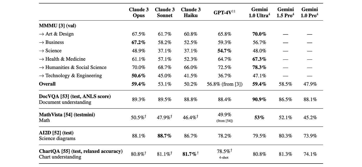
Imagine you were tasked to build a system that could answer incoming queries correctly while minimizing cost. What approach would you take?
Your first intuition might be to develop something called a “LLM cascade” which is exactly what is proposed in both the FrugalGPT and AutoMix papers.
In an LLM cascade you pass a query to the least expensive LLM you have, then ask that same model if the query was answered adequately. If the small model judged that it’s own answer was correct, then you return the answer from the small model to the user. If the small model’s answer was not deemed correct, you try the same process with a larger model.

This approach can be practical because smaller models can be much, much less expensive than larger models.
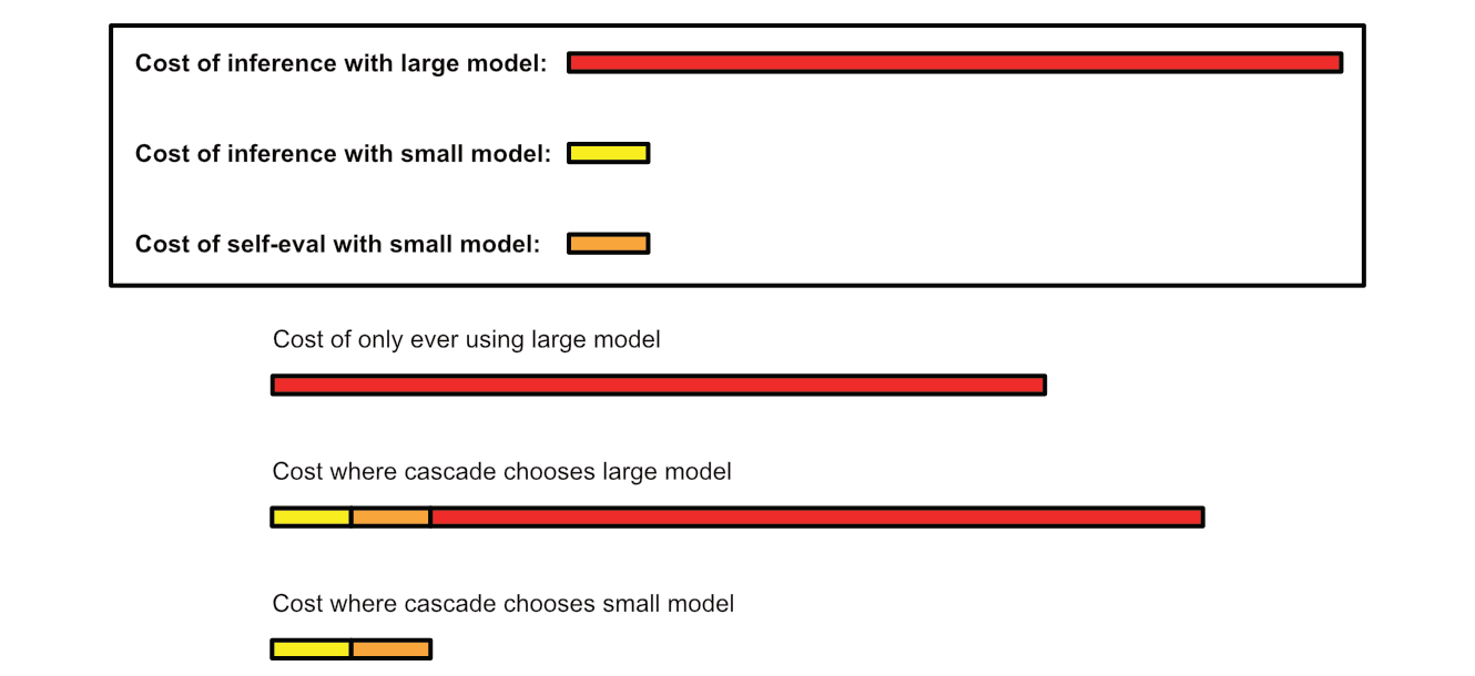
Naturally, an LLM cascade is very dependent on both the users queries and the models chosen, which is where the simplicity of the approach can be a tremendous asset. Because there is no training involved it’s incredibly easy to set up and modify a cascade at will.
If you can whip this up in 5 minutes and see a 10x reduction in LLM inference cost with negligible performance impact, then that’s pretty neat. However, an issue with this simple approach is that you are likely to see a significant performance drop.
The issue lies in self-evaluation. A lot of the time our smaller language model will be able to tell if it got the answer wrong, but sometimes the smaller model won’t be able to detect its own mistakes.

Because LLM cascades rely on self-evaluations to decide whether to continue to a larger model or return the current response, a poor self-evaluation can significantly inhibit the quality of the final output. AutoMix employs something called a “Partially Observable Markov Decision Process” based on “Kernel Density Estimation” to alleviate this problem. Let’s unpack those ideas:
A High-Level Intro to POMDPs
A “Partially Observable Markov Decision Process” (POMDP) is an extension of something called a “Markov Decision Process” (MDP).
A Markov Decision Process (MDP) is a way of modeling the types of states a system can be in, and the actions that system can take to transition between states. Say you have a robot, for instance, and you want to allow that robot to navigate through an environment.
You can construct a graph of the possible states that robot can occupy, as well as the cost to transition between states.
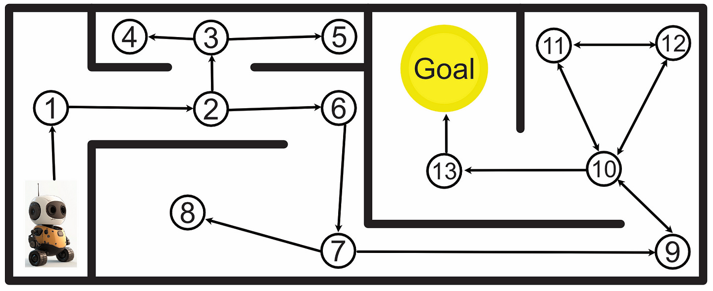
Once the graph is set up, you can analyze that graph to calculate the best course of action.
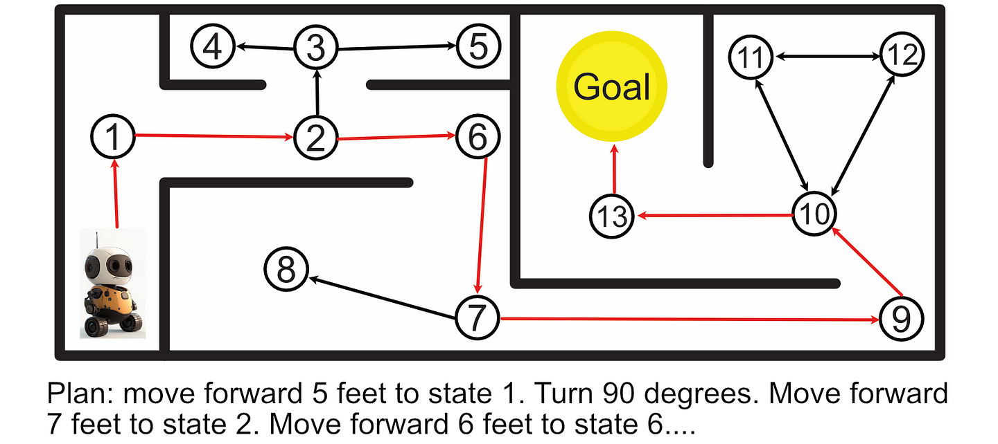
This is called a “Markov Decision Process”, and is a super powerful tool in modeling complex systems.
One problem with a classic Markov Decision Process is instability. Imagine we tell our robot to follow the plan to reach the goal, and then the robot’s wheel slips halfway down a hallway; resulting in the robot turning slightly. If we continue executing our pre-defined instructions as before, the robot will get stuck in a corner rather than reach its destination.
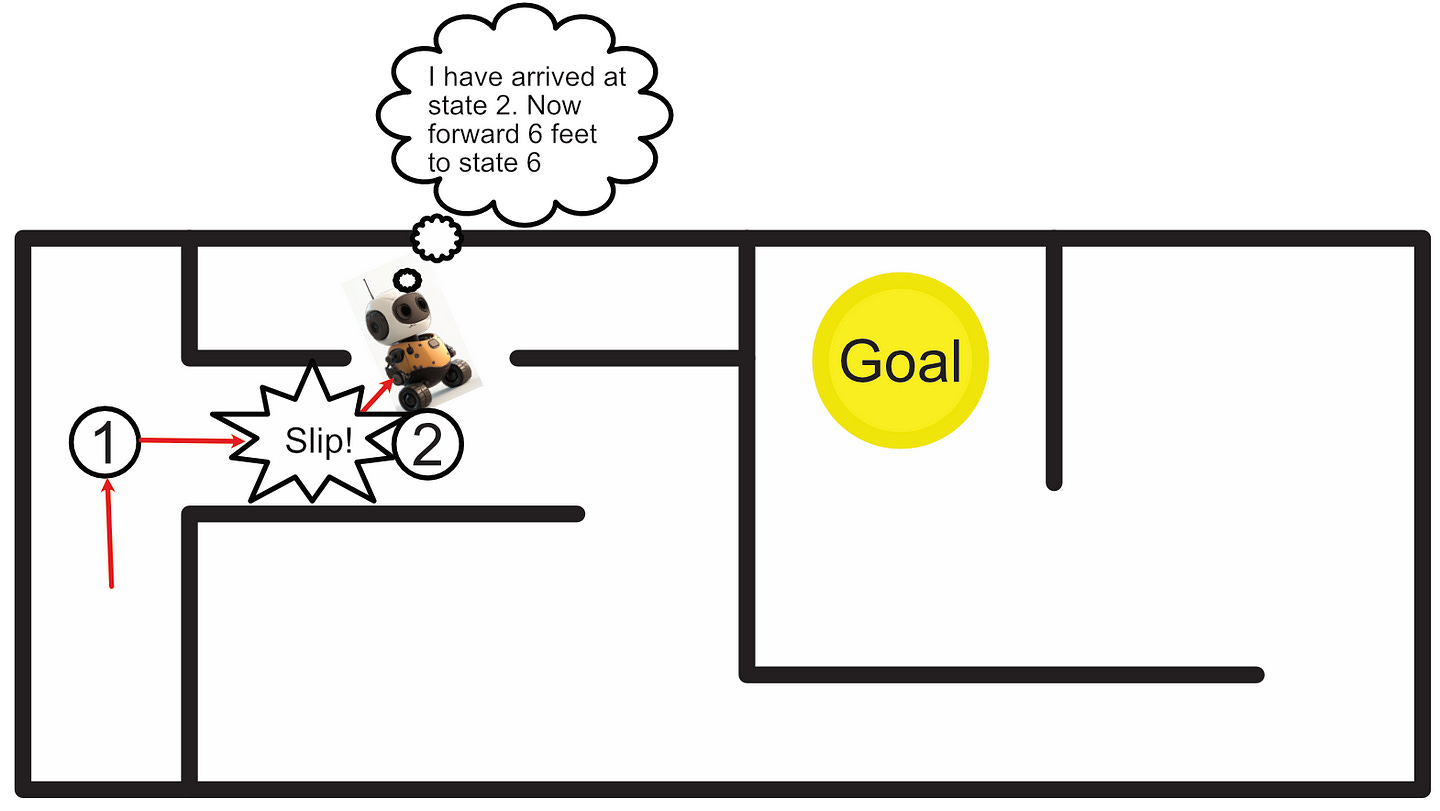
“Partially Observable” Markov Decision Processes (POMDP) are designed to alleviate this problem. The idea of a POMDP is that we assume we never know the true state of the robot, but rather we can make observations and form a probabilistic belief about the state of the system.
If we slap some sensors on our robot, and have it navigate our environment, we can use our sensors to check if we think the robot has ended up in the correct spot. The sensor might not be able to perfectly identify where we are, but we can use our best guess to make a reasonable decision.
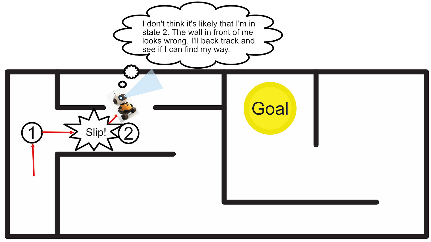
Let’s explore how AutoMix employs POMDP’s to support the LLM Cascade. In doing so, we’ll explore some of the inner workings of POMDP’s more in depth.
AutoMix’s POMDP Supported LLM Cascade
Full Code for the AutoMix Portion of this article can be found here
Recall that an LLM Cascade uses self evaluation to either return the response from a smaller language model or pass the prompt to a larger model.

The main idea of AutoMix is, instead of taking the self-evaluations of a model at face value, we turn them into a probabilistic “observation” which hints at the performance of the LLM, then we use that probabilistic observation to decide what action we should take.
To turn a binary “yes or no” self-evaluation into a probability, the authors of AutoMix ask the language models to self-evaluate numerous times with a high temperature setting. Temperature increases how erratic a language models responses are by allowing an LLM to accept output that is occasionally less optimal. If we choose a very high temperature rating, and ask the model to self-evaluate a few times, it allows us to build a probability distribution of self evaluation based on how many times the model says the answer was acceptable or not.
First, we can use langChain’s with_structured_output to get a binary true or false evaluation for if an LLM thinks the answer is correct.
"""Creating an "evaluator" using langchain's "with_structured_output".
Basically, this function defines a class which represents the data we want from
the LLM (SelfEval), then langchain uses that class to format the LLMs response into a true
or false judgement of if the model was accurate or not. This allows us to ask an LLM if an
answer was correct or not, and then get back a boolean.

I also have the model form a rationale, before constructing the boolean, serving as a form of
chain of thought.

we specify a high temperature, meaning using an evaluator multiple times
can result in a distribution of evaluations due to high model randomness
"""

from typing import TypedDict
from langchain_openai import ChatOpenAI
from langchain_core.prompts import ChatPromptTemplate

def create_evaluator(model):

    #Defines the structure of the output
    class SelfEval(TypedDict):
        rationale: str
        judgement: bool

    #The system prompt provided to the model
    #prompt lightly modified from AutoMix paper
    self_eval_prompt = ChatPromptTemplate.from_messages(
        [
            (
                "system",
                """Instruction: Your task is to evaluate if the AI Generated Answer is correct or incorrect based on the
provided context and question. Provide ultimate reasoning that a human would be satisfied with, then choose between
Correct (True) or Incorrect (False).
                """,
            ),
            ("placeholder", "{messages}"),
        ]
    )

    #creating a lang chang that outputs structured output
    evaluator = self_eval_prompt | ChatOpenAI(
        model=model, temperature=1 #setting a high temperature
    ).with_structured_output(SelfEval)

    return evaluator
Then we can have a model answer some question
"""Having an LLM answer a riddle

There was a plane crash in which every single person was killed.
Yet there were 12 survivors. How?
"""

from openai import OpenAI

model = 'gpt-3.5-turbo'

context = """There was a plane crash in which every single person was killed. Yet there were 12 survivors. How?"""
question = "Solve the riddle"

client = OpenAI(api_key=api_key)
response = client.chat.completions.create(
        model=model,
        messages=[
            {"role": "user", "content": f"context:\n{context}\n\nquestion:\n{question}"}
            ],
    )

answer = response.choices[0].message.content.strip()
We can use the evaluator we defined to ask the model to evaluate it’s own answer a few times, and construct a normal distribution based on how many true and false self evaluations there were.
""" Constructing a normal distribution (a.k.a. bell curve, a.k.a gaussian),
based on 40 self evaluations, showing how likely an answer was right or
wrong based on several LLM self-evaluations.

Gaussians have two parameters:
- the mean, or center of the distribution: calculated as just the average value
- the standard deviation: which is how spread out the values are.

The funciton `gaussianize_answer` runs self eval some number of times,
gets a distribution of self evaluations saying the response was good
or poor, then constructs a gaussian describing that overall distribution.
"""

import numpy as np
import matplotlib.pyplot as plt
from scipy.stats import norm

def gaussianize_answer(context, question, answer):
    num_evaluations = 40
    evaluations = []
    evaluator = create_evaluator(model)

    for _ in range(num_evaluations):

        for i in range(2):
            #allowing the evaluator to make several attempts at judgements
            #and wrapping it in a try/catch to deal with the odd parsing error.
            try:
                evaluation = evaluator.invoke({"messages": [("user", f"""Context: {context}
            Question: {question}
            AI Generated Answer: {answer}""")]})

                evaluations.append(evaluation['judgement'])
                break
            except KeyboardInterrupt as e:
                raise e
            except:
                print('evaluator error')
        else:
            print('too many errors, skipping evaluation step')

    # Calculate probability (mean) of evaluations
    probability = sum(evaluations) / len(evaluations)

    # Calculating mean and standard deviation, which define a gaussian
    mean = probability
    std_dev = np.sqrt(probability * (1 - probability) / len(evaluations))

    return mean, std_dev

mean, std_dev = gaussianize_answer(context, question, answer)

#cant draw gaussian if there's perfect consensus
if mean != 0 and mean !=1:
    # Create a range for x values
    x = np.linspace(0, 1, 100)
    y = norm.pdf(x, mean, std_dev)

    # Plot the Gaussian
    plt.plot(x, y, label=f'Gaussian Distribution\nMean={mean:.2f}, Std Dev={std_dev:.2f}')
    plt.title("Gaussian Distribution of True Value Probability")
    plt.xlabel("Probability")
    plt.ylabel("Density")
    plt.legend()
    plt.show()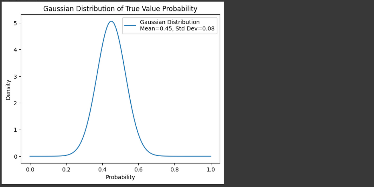
Without using a POMDP, one could simply apply a threshold to these probabilities and use them to make decisions about how to navigate through the cascade, possibly seeing an improvement over using individual self evaluation results. However, self evaluations are know to be noisy and unreliable. Let’s do some self-evaluations on several answers and overlay the distributions of correct and incorrect answers to explore just how noisy self-evaluation can be:
"""Creating normal distributions based on self evaluations for a few answers.
Recall that the riddle was the following:

There was a plane crash in which every single person was killed. Yet there were 12 survivors. How?
"""

#A selection of a few hardcoded LLM answers
llm_answers = []
#correct
llm_answers.append("The 12 survivors were married couples.")
llm_answers.append("The people on the plane were all couples - husbands and wives.")
llm_answers.append("The answer to this riddle is that the 12 survivors were married couples.")

#incorrect
llm_answers.append("The riddle is referring to the survivors being the 12 months of the year.")
llm_answers.append("The riddle is referring to the survivors as the numbers on a clock (numbers 1-12). So, the answer is that the \"12 survivors\" are actually the numbers on a clock.")

#evaluating all answers
distributions = []
for llm_answer in llm_answers:
    mean, std = gaussianize_answer(context, question, llm_answer)
    distributions.append((mean, std))
Here, the first three answers are correct answers to the riddle, while the final two answers are incorrect answers to the riddle. We can plot these distributions to see how well our auto-evaluation strategy can separate good and bad answers.
"""Plotting the gaussians we created in the previous code block.
Correct answers are dotted, wrong answers are solid.
"""

fig = plt.figure(figsize=(10, 6))

#plotting all gaussians
for i, dist in enumerate(distributions):
    #unpacking tuple
    mean, std = dist

    name = f'LLM answer {i}'

    #labeling the two clearly wrong answers as dotted lines (i=3 and i=4)
    if i>=3:
        stroke = '-'
    else:
        stroke=':'

    if std == 0:
        plt.plot([mean,mean],[0,1], linestyle=stroke, label=name)
    else:
        # Create a range for x values
        x = np.linspace(0, 1, 100)
        y = norm.pdf(x, mean, std)
        plt.plot(x, y, linestyle=stroke, label=name, alpha=0.5)
plt.title("Gaussian Distribution of True Value Probability Across Answers")
plt.xlabel("Probability")
plt.ylabel("Density")
plt.legend()
plt.show()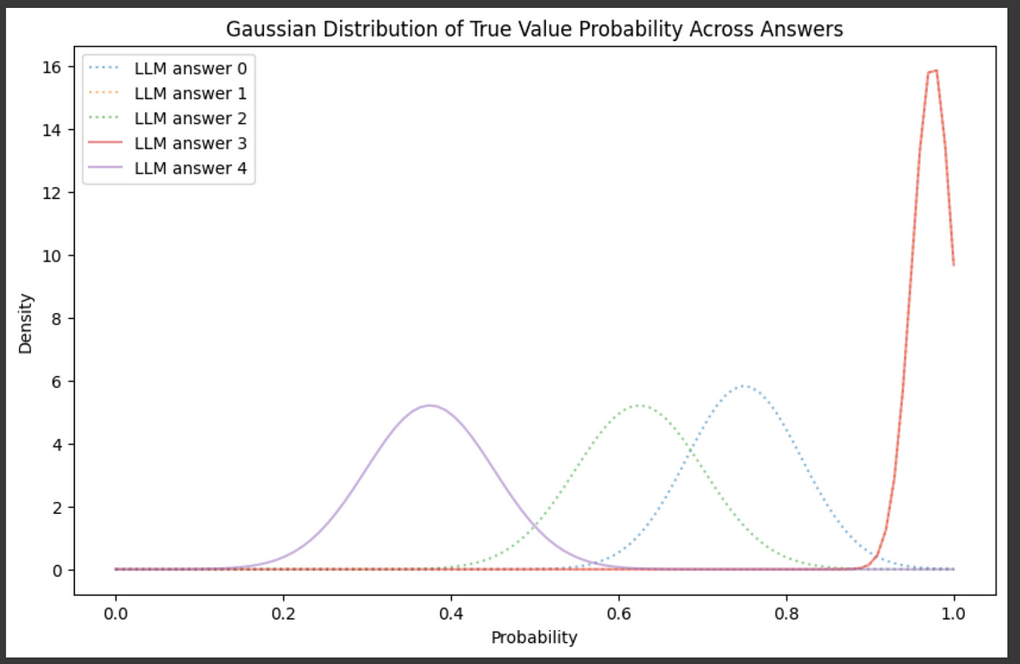
And… It did a pretty bad job. The distributions for good and bad answers are all mixed up. Language models are frustratingly bad at knowing if their own answers are wrong or not. If we use this self-evaluation strategy as-is, our LLM cascade will likely make wrong decisions; sometimes triggering expensive models when it shouldn't and sometimes returning bad responses when it shouldn’t.
This is where the “partially observable” aspect of POMDPs comes in. Instead of assuming the self-evaluations we’re constructing are accurate, we can treat it like an observation and use that observation to try to predict if an answer is really good or not.
In the AutoMix paper they do that through a process called Kernel Density Estimation (KDE). Say you have a model, and you have a handful of examples where you know the model answered the question correctly and incorrectly. You can do self-eval on question-answer pairs to figure out where self-evaluations typically end up when the models answer is actually correct or incorrect.
In other words, we’re going to build a dataset of self-evaluation scores where we know the model’s answer is right, and another set where we know the models answer is wrong, then we’re going to use that data to make routing decisions.
Here I’m constructing a synthetic dataset of self-evaluations for correct and incorrect answers, but you might imagine running the gaussianize_answer function we previously defined on a bunch of questions and answers to create this dataset.
import numpy as np
import matplotlib.pyplot as plt
import pandas as pd
import seaborn as sns

# Creating a synthetic dataset with self evaluation results
# and actual performance results.
np.random.seed(0)

n_each = 50

selfeval_bad = np.random.normal(0.55, 0.05, n_each)    # Lower confidence around 0.4
selfeval_good_1 = np.random.normal(0.9, 0.03, n_each)  # Higher confidence around 0.7
selfeval_good_2 = np.random.normal(0.6, 0.03, n_each)  # Higher confidence around 0.6
selfeval_good = np.concatenate([selfeval_good_1, selfeval_good_2]) #combining both good distributions
self_eval = np.concatenate([selfeval_good_1, selfeval_good_2, selfeval_bad])
true_performance = [1] * (n_each*2) + [0] * n_each

#plotting a swarm plot
df = pd.DataFrame()
df['true_performance'] = true_performance
df['self_eval'] = self_eval

ax = sns.swarmplot(x="true_performance", y="self_eval", data=df)
plt.title("Training Dataset with True Performance vs Self Evaluation")

plt.show()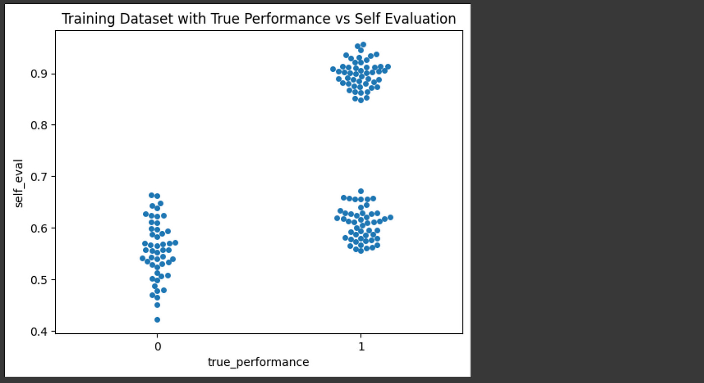
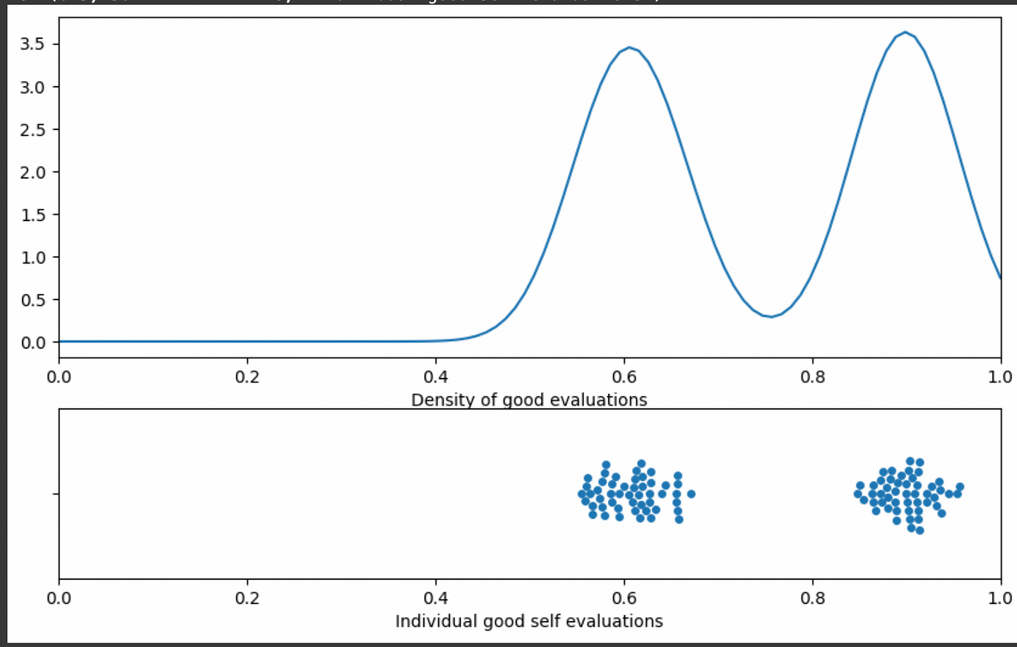
The idea of kernel density estimation (KDE) is to turn these individual examples into smooth density distributions such that we can use them to calculate the probability of a truly good answer. In other words, we want to be able to say “I know self-eval said there was a 50% chance the answer is good, but based on a dataset of self-evaluations I know that almost certainly means the answer is wrong because bad answers at a self evaluation of 0.5 are way more dense than good answers at 0.5”. KDEs allow us to do that.
To construct a KDE you first put a gaussian (a.k.a. kernel, a.k.a bell curve) on every point in a distribution:
"""Placing a gaussian with an average value equal to every point
in the distribution of self evaluation results for good predictions
The standard deviation can be modified as necessary. Here I'm defining the
standard deviation as 0.05 for all gaussians, but they could be larger
or smaller, resulting in smoother or more sensitive KDEs
"""

import matplotlib.gridspec as gridspec
from scipy.stats import norm

fig = plt.figure(figsize=(10, 6))

# Creating a gaussian distribution with a small deviation on every point in a set of data
gs = gridspec.GridSpec(2, 1, height_ratios=[2, 1])
ax1 = fig.add_subplot(gs[0])
std = 0.05
for mean in selfeval_good:
    x = np.linspace(0, 1, 100)
    y = norm.pdf(x, mean, std)
    plt.plot(x,y)
plt.xlim([0, 1])
plt.xlabel("Gaussians built on good evaluations")

ax2 = fig.add_subplot(gs[1])
sns.swarmplot(x = 'self_eval', data = df[df['true_performance']==1])
plt.xlim([0, 1])
plt.xlabel("Individual good self evaluations")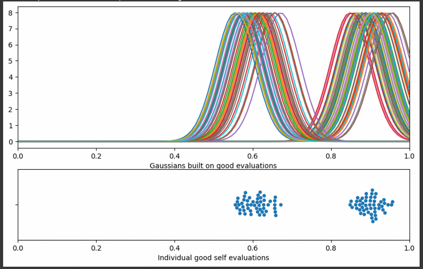
Then we can add them all up to create a smooth volume of predictions. The more predictions there are in a region, the larger the volume is.
"""modifying the code of the previous code block. Instead of saving
many gaussians, each gaussian is added to the same vector of values
In other words, wer're stacking all the gaussians on top of eachother
"""

import matplotlib.gridspec as gridspec
fig = plt.figure(figsize=(10, 6))

# Creating a gaussian distribution with a small deviation on every point in a set of data
gs = gridspec.GridSpec(2, 1, height_ratios=[2, 1])
ax1 = fig.add_subplot(gs[0])
std = 0.05
y = np.zeros(100)
for mean in selfeval_good:
    x = np.linspace(0, 1, 100)
    y += norm.pdf(x, mean, std)
plt.plot(x,y)
plt.xlim([0, 1])
plt.xlabel("Sum of all gaussians built on all good evaluations")

ax2 = fig.add_subplot(gs[1])
sns.swarmplot(x = 'self_eval', data = df[df['true_performance']==1])
plt.xlim([0, 1])
plt.xlabel("Individual good self evaluations")In this graph the y axis doesn’t really mean anything. The more data you have, the taller this graph will be, meaning the y axis is dependent on both density and the number of total predictions. Really, we’re just interested in density, so we can calculate the area under the curve of the sum of gaussians then divide by that area. That will mean, regardless of how many predictions you have the area under the curve will always be 1, and the height of the curve will be the relative density of one region vs another, rather than being influenced by the number of samples you have.
"""Modification of the previous code block to create a density plot
Calculating the area under the curve, then dividing the values
by that area. This turns a vague volume of results into a density
distribution, essentially getting rid of the impact that larger numbers
of samples tend to make the y axis taller.
"""

import matplotlib.gridspec as gridspec
fig = plt.figure(figsize=(10, 6))

# Creating a gaussian distribution with a small deviation on every point in a set of data
gs = gridspec.GridSpec(2, 1, height_ratios=[2, 1])
ax1 = fig.add_subplot(gs[0])
std = 0.05
y = np.zeros(100)
for mean in selfeval_good:
    x = np.linspace(0, 1, 100)
    y += norm.pdf(x, mean, std)

#converting to density (total area under the curve, regardless of the number
#of samples, will be equal to 1. Densities beteen distributions are comperable even
#if the number of samples are different)
area_under_curve = np.trapz(y, dx=1/100)
y = y/area_under_curve

plt.plot(x,y)
plt.xlim([0, 1])
plt.xlabel("Density of good evaluations")

ax2 = fig.add_subplot(gs[1])
sns.swarmplot(x = 'self_eval', data = df[df['true_performance']==1])
plt.xlim([0, 1])
plt.xlabel("Individual good self evaluations")
And thus we’ve constructed a KDE. I know I’ve been throwing terms around like crazy , so I want to take a moment to reiterate what this graph represents.
We start with a bunch of answers to questions by an LLM, and we get each of those dots in the graph above by asking the LLM to self evaluate a few times with a high temperature on the same question and answer, turning each answer into a probability. Self-evaluations are often noisy and inconsistent, so what we would like to do is find what self-evaluation scores are the most likely to actually correspond to a correct answer. To do that, we’re looking at the self-evaluation scores of actually good answers, and finding the region in which self-evaluation scores are more dense. If we have a self evaluation score which lies in a region where there is a high density of actual good answers, then it’s probably more likely to be a good self-evaluation.
All that code we made to construct the kernel density estimation can be replaced with scipy.stats.gaussian_kde. We can use that function for the self evaluation of both truly good answers and truly bad answers to get an idea of which self-evaluation values are more likely given a good or bad answer.
from scipy.stats import gaussian_kde

# Perform KDE for each performance state
good_kde = gaussian_kde(selfeval_good, bw_method=0.3)
poor_kde = gaussian_kde(selfeval_bad, bw_method=0.3)

# Define a range of confidence scores for visualization
confidence_range = np.linspace(0, 1.0, 200)

# Evaluate KDEs over the range of confidence scores
good_density = good_kde(confidence_range)
poor_density = poor_kde(confidence_range)

# Plot the KDE for each performance state
plt.figure(figsize=(10, 6))
plt.plot(confidence_range, poor_density, label="Density of Self Eval for Poor Results")
plt.plot(confidence_range, good_density, label="Density of Self Eval for Good Results")
plt.title("KDE of Confidence Scores for Good and Poor Performance")
plt.xlabel("Confidence Score Through Self Evaluation")
plt.ylabel("Density of Predictions")
plt.legend()
plt.show()So, if we had a self evaluation of 60%, for instance, we could calculate the probability of if it would actually be a good answer by comparing the relative densities of good and bad answers in that region.
# Plot the KDE for each performance state
plt.figure(figsize=(10, 6))
plt.plot(confidence_range, poor_density, label="Density of Self Eval for Poor Result", alpha=0.7)
plt.plot(confidence_range, good_density, label="Density of Self Eval for Good Result", alpha=0.7)

#plotting the probabilities of good or bad at a given location
sample_confidence = 0.6
conf_poor = poor_kde(sample_confidence)[0]
conf_good =  good_kde(sample_confidence)[0]
label = f'Good Probability: {int(conf_good/(conf_poor+conf_good)*100)}%'
plt.plot([sample_confidence]*3,[0,conf_poor, conf_good], 'r', linewidth=3, label=label)
plt.plot([sample_confidence]*2,[conf_poor, conf_good], 'r', marker='o', markersize=10)

plt.title("KDE of Confidence Scores for Good and Poor Performance States")
plt.xlabel("Confidence Score Through Self Evaluation")
plt.ylabel("Density of Predictions")
plt.legend()
plt.show()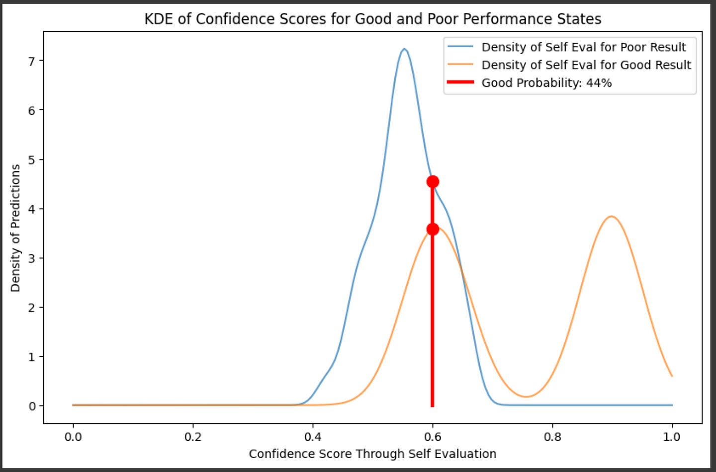
We can sweep through the entire x axis and calculate the probability that an answer is good, based on the ratio of densities of the known training data, across all possible self-evaluation results
plt.figure(figsize=(10, 6))
plt.title("Probability that the prediction is correct based on the difference of the self evaluation distributions")
good_probability = np.array([good/(good+poor) for (good, poor) in zip(good_density, poor_density)])
plt.plot(confidence_range, good_probability)
plt.xlabel("Confidence Score Through Self Evaluation")
plt.ylabel("Probability Correct")
This is pretty nifty, but you might notice a problem. At a self-evaluation score of 0.2, for instance, the probability (based on the ratio of densities) is 100% not because there are a lot of examples of good predictions at that point, but because there aren’t any samples in that region.
To deal with this, the AutoMix paper also talks about constructing a KDE across all the data, and only keeping results that have self-evaluations that lie within dense regions of the dataset.
"""Creating a graph of probability that an answer is right
and also a graph of the density of all the training data
"""

import matplotlib.gridspec as gridspec
fig = plt.figure(figsize=(10, 6))

total_kde = gaussian_kde(self_eval, bw_method=0.3)
total_density = total_kde(confidence_range)
height_normalized_total_density = total_density/max(total_density)
confidence_threshold = 0.5
density_threshold = 0.1

#marking
gs = gridspec.GridSpec(2, 1, height_ratios=[2, 1])
ax1 = fig.add_subplot(gs[0])
plt.plot(confidence_range, good_probability)
threshold = 0.5
plt.fill_between(confidence_range, good_probability, 0, where=(good_probability > confidence_threshold), color='blue', alpha=0.2, label=f'Probability based on density ratios > {confidence_threshold}')
plt.ylabel("Probability Correct")
plt.legend()

ax2 = fig.add_subplot(gs[1])
plt.plot(confidence_range, height_normalized_total_density, label="Normalized density of all self evaluations", alpha=1)
plt.fill_between(confidence_range, height_normalized_total_density, 0, where=(height_normalized_total_density > density_threshold), color='blue', alpha=0.2, label=f'Total normalized density > {density_threshold}')
plt.xlabel("Confidence Score Through Self Evaluation")
plt.ylabel("Density of Predictions")
plt.legend()
plt.show()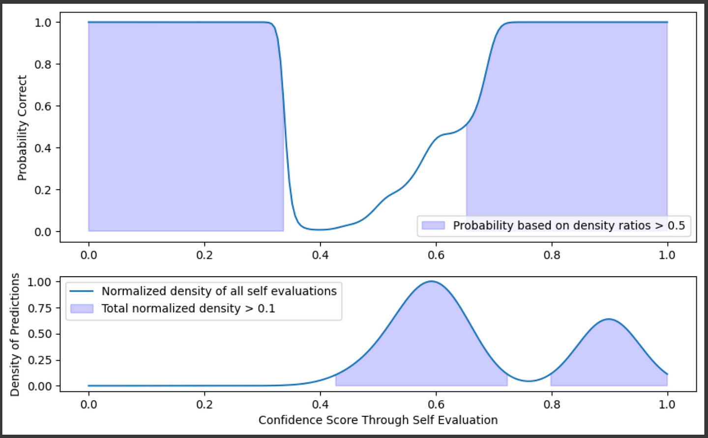
So, we can say a self-evaluation is good if the probability of a prediction is good and if the self evaluation exists within a region where there is a fair amount of training data. Even though the probability might be high at 0.2, we know there’s no data at that point, so we would be skeptical of that self-evaluation.
With LLMs, there is generally a tradeoff between cost and performance. We might be willing to accept different probabilities that an answer is good depending on the cost and performance constraints of our use case. We can balance cost and performance by changing the threshold at which we decide to call the larger LLM given a smaller LLM’s self-evaluation.
"""Rendering a gradient of cost/performance tradeoff over the graphs
"""

import matplotlib.gridspec as gridspec
fig = plt.figure(figsize=(10, 6))

total_kde = gaussian_kde(self_eval, bw_method=0.3)
total_density = total_kde(confidence_range)
height_normalized_total_density = total_density/max(total_density)
confidence_threshold = 0.5
density_threshold = 0.1

cost_based_thresholds = [0.0,0.1,0.2,0.3,0.4,0.5,0.6,0.7,0.8,0.9]

#marking
gs = gridspec.GridSpec(2, 1, height_ratios=[2, 1])
ax1 = fig.add_subplot(gs[0])
plt.plot(confidence_range, good_probability)
threshold = 0.5

threshold = cost_based_thresholds[0]
plt.fill_between(confidence_range, good_probability, 0, where=(np.logical_and(good_probability > threshold, height_normalized_total_density > density_threshold)), color='red', alpha=0.2, label=f'bound by cost')

for threshold in cost_based_thresholds[1:-2]:
    plt.fill_between(confidence_range, good_probability, 0, where=(np.logical_and(good_probability > threshold, height_normalized_total_density > density_threshold)), color='red', alpha=0.2)

threshold = cost_based_thresholds[-1]
plt.fill_between(confidence_range, good_probability, 0, where=(np.logical_and(good_probability > threshold, height_normalized_total_density > density_threshold)), color='red', alpha=1, label=f'bound by performance')

plt.ylabel("Probability Correct")
plt.legend()

ax2 = fig.add_subplot(gs[1])
plt.plot(confidence_range, height_normalized_total_density, label="Normalized density of all self evaluations", alpha=1)
for threshold in cost_based_thresholds:
    plt.fill_between(confidence_range, height_normalized_total_density, 0, where=(np.logical_and(good_probability > threshold, height_normalized_total_density > density_threshold)), color='red', alpha=0.2)
plt.xlabel("Confidence Score Through Self Evaluation")
plt.ylabel("Density of Predictions")
plt.legend()
plt.show()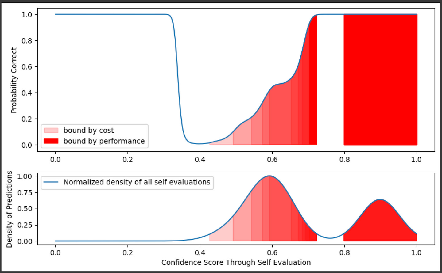
So, based on training data we created of self-evaluations, paired with annotations of if the answers that were self-evaluated were good or bad, we can build a probability distribution of if the answer is actually good or bad, and have a degree of confidence based on the density of our training data within that region. We can use this data to make decisions, thus allowing us to make “observations” about what we think our true performance likely is.
I’ll be skipping some fairly verbose code. Feel free to check out the full code:
MLWritingAndResearch/AutoMix.ipynb at main · DanielWarfield1/MLWritingAndResearch
Notebook Examples used in machine learning writing and research - MLWritingAndResearch/AutoMix.ipynb at main ·…github.com
Imagine we have three LLMS with different abilities to self-evaluate.
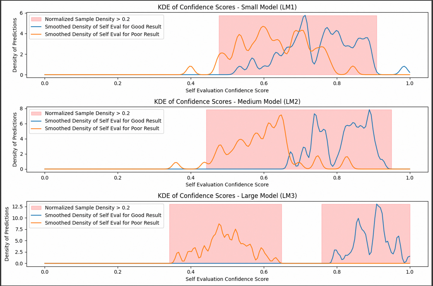
Based on this data, you could use this information to say “I have __% confidence that this answer is actually correct, based on a comparison of a given self evaluation with a dataset of self-evaluations on answers of known quality.”

We can feed a query to our tiniest model, have it self-evaluate, and decide if the self evaluation is good enough based on our KDEs for that model. If it’s not, we can move onto a bigger model. We do that until we’re happy with our output.
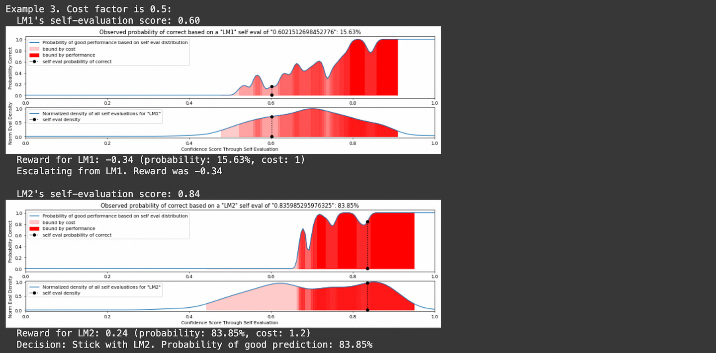
You might notice text about “reward” and “cost” in that output. In LLM routing there’s a fundamental tradeoff between performance and cost. If you want better performance it’ll be more expensive. If you want lower cost you need to deal with less performance. AutoMix uses the parameter λ (lambda) to control that tradeoff.
We want to consistently achieve high performance at a low cost, but are willing to balance between the two based on λ. If we care more about performance we might use a small λ value, and if we care more about cost we might choose a large λ value. This tradeoff is defined in the reward function:

This can actually get pretty complicated. Formally, in a POMDP we need to account for all probabilities and all costs of all models when making a decision. I’m planning on tackling POMDPs more in depth at some point in the future, and this article has taken long enough to come out, so I simply made the reward function equal to the probability of the current output being good minus λ times the cost of the next model. So, instead of looking at all possibilities of all future models, I’m simply saying “is the current output good enough vs the cost to try again with the next model, based on λ”.
Again, full code can be found here.
"""Constructing the POMDP and running it with simulated inferences
This is a simplification of the POMDP which just looks at the probability
of the current self evaluation and the cost of the next model.
"""
class Model:
    def __init__(self, name, kde_good, kde_poor, kde_density, good_threshold, cost):
        """
        Initialize each model with KDEs for good/poor predictions, a good_threshold for trusting its output,
        and a cost associated with using this model.
        """
        self.name = name
        self.kde_good = kde_good
        self.kde_poor = kde_poor
        self.kde_density = kde_density
        self.good_threshold = good_threshold
        self.cost = cost

    def evaluate(self, self_eval, density_threshold=0.2):
        """Calculate the probability that the prediction is good based on the self evaluation score."""
        prob_good = observe_good_probability(self_eval, self.kde_good, self.kde_poor, self.kde_density,
                                             normalized_density_threshold=density_threshold, model_name=self.name, plot=True)
        plt.show()
        return prob_good


class POMDP:
    def __init__(self, models, lambda_param=0.1):
        """
        Initialize the POMDP with a list of models and the lambda parameter that balances performance vs. cost.
        """
        self.models = models
        self.lambda_param = lambda_param  # Parameter to balance cost vs. performance in reward function

    def compute_reward(self, prob_good, cost):
        """
        Compute the reward based on the performance (prob_good) and the cost of the model.
        """
        return prob_good - self.lambda_param * cost

    def run_simulation(self, n_examples=5):
        """Run the POMDP decision process across multiple examples."""
        for example in range(n_examples):
            print(f"Example {example + 1}. Cost factor is {self.lambda_param}:")
            for model_iter, model in enumerate(self.models):
                self_eval = np.random.uniform(0.6, 1.0)  # Generate a random self-evaluation score
                print(f"  {model.name}'s self-evaluation score: {self_eval:.2f}")
                prob_good = model.evaluate(self_eval)

                # Compute reward based on the current model's performance and cost
                if model_iter<len(self.models)-1:
                    reward = self.compute_reward(prob_good, self.models[model_iter+1].cost)
                    print(f"  Reward for {model.name}: {reward:.2f} (probability good: {prob_good*100:.2f}%, cost of next: {self.models[model_iter+1].cost})")
                else:
                    reward = 1 #no more models to escelate to

                # Decision: Should we trust this model or escalate?
                if reward > 0:  # If the reward is positive, we trust the model
                    print(f"  Decision: Stick with {model.name}. Probability of good prediction: {prob_good*100:.2f}%\n")
                    break  # Stop traversing as we trust this model
                else:
                    print(f"  Escalating from {model.name}. Reward was {reward:.2f}\n")
            else:
                print("  No suitable model found, escalating failed.\n")


# Define models dynamically with their respective KDEs, thresholds, and costs
lm1 = Model("LM1", kde_good_lm1, kde_poor_lm1, kde_density_lm1, good_threshold=0.8, cost=1)
lm2 = Model("LM2", kde_good_lm2, kde_poor_lm2, kde_density_lm2, good_threshold=0.85, cost=1.2)
lm3 = Model("LM3", kde_good_lm3, kde_poor_lm3, kde_density_lm3, good_threshold=0.9, cost=1.5)

# Initialize the POMDP with the list of models and the lambda parameter (balancing performance vs cost)
pomdp = POMDP(models=[lm1, lm2, lm3], lambda_param=0.5)

# Run the simulation
pomdp.run_simulation(n_examples=5)
And here’s a few examples of it in action:
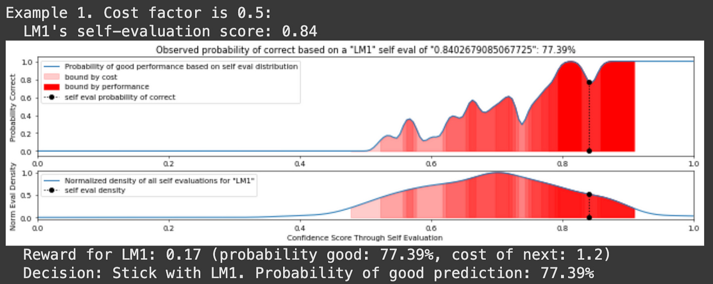
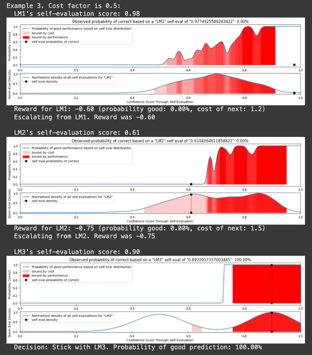
And, ta-da, we have made an AutoMix style POMDP that allows us to balance cost and performance tradeoffs by routing to different LLMs in a cascade. Let’s check out a different example of LLM Routing which approaches the problem in a few different ways.
A Few Approaches from RouteLLM
The Route LLM paper presents a few compelling approaches to LLM Routing:
Similarity Weight Ranking
Matrix Factorization
BERT Classification
Causal LLM Classification
We’re going to focus on Similarity Weight Ranking and BERT Classification in this article, but before we dive in I’d like to talk about how RouteLLM differs from AutoMix in terms of the data it uses.
RouteLLM: A Different Approach to Data
The AutoMix approach we discussed previously focuses on being able to whip up an LLM router with very little data. With only a few tens, or perhaps hundreds, of examples of questions and answers you can use that data to build out density estimations and develop AutoMix. This is incredibly powerful because, starting from just a few LLMs and a dream, you can create all the data necessary to build AutoMix by yourself in an afternoon.
RouteLLM takes a much more “big data” approach to LLM Routing by building sophisticated models which make intricate routing decisions. This is a double-edged sword: You might end up with heightened performance, but at an additional cost to get things set up.
Instead of looking at self-evaluation results, like what is done in AutoMix, RouteLLM analyzes the query itself and attempts to make decisions based on which models are better at certain types of queries. To make this more nuanced assessment, they use a ton of data. Specifically:
The bulk of the data used in RouteLLM is 80k examples of human preference data from chatbot arena, which allows humans to rank the relative performance of two random LLMs with one another on a given query.
They use the multiple choice dataset MMLU to automatically evaluate if a model was correct or incorrect, with a high degree of certainty, on a given prompt
The Nectar dataset contains GPT-4’s ranking of several smaller models responses.
The data pre-processing of RouteLLM is a fascinating topic, which we’ll briefly discuss before getting into how they actually create routers.
Code for the RouteLLM exploration is available here
Turning Sparse Preference Data into Routing Data
The primary dataset used in the RouteLLM paper is from “Chatbot Arena”. Chatbot arena allows users to ask a question to multiple chatbots and rate which one they find to be the best answer to the query. The RouteLLM paper uses this to train a model for routing.
Keep reading with a 7-day free trial
Subscribe to Intuitively and Exhaustively Explained to keep reading this post and get 7 days of free access to the full post archives.


