Multi-Headed Self Attention — By Hand

Hand computing the cornerstone of modern AI

“Focus” By Daniel Warfield using MidJourney. All images by the author unless otherwise specified. Article originally made available on Intuitively and Exhaustively Explained.

Multi-Headed Attention is likely the most important architectural paradigm in machine learning. This summary goes over all critical mathematical operations within multi-headed self attention, allowing you to understand it’s inner workings at a fundamental level. If you’d like to learn more about the intuition behind this topic, check out the IAEE article.

---

Transformers — Intuitively and Exhaustively Explained

---

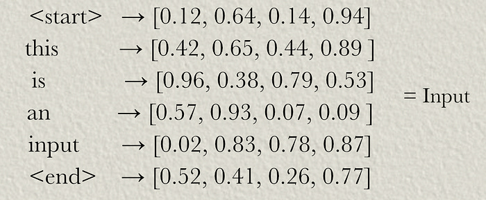
Step 1: Defining the Input

Multi-headed self attention (MHSA) is used in a variety of contexts, each of which might format the input differently. In a natural language processing context one would likely use a word to vector embedding, paired with positional encoding, to calculate a vector that represents each word. Generally, regardless of the type of data, multi-headed self attention expects of sequence of vectors, where each vector represents something.

An example of the input one might expect when applying MHSA in a language modeling context.

Step 2: Defining the Learnable Parameters

Multi headed self attention essentially learns three weight matrices. These are used to construct the “query”, “key”, and “value”, which are used later in the mechanism. We can define some weight matrices to use in this example which represent learned parameters of the model. These would be initially randomly define, and then update throughout the training process.

Step 3: Defining the Query, Key, and Value

Now that we have weight matrices for our model, we can multiply them by the input to generate our query, key, and value. Recall that in matrix multiplication, every value in a row of the first matrix is multiplied by the corresponding values in a column in the second matrix. Those multiplied values are summed to represent one value in the output.

The same operations are used to construct the key and value matrices, and thus we’ve constructed the query, key, and value

Step 4: Dividing into Heads

In this example we’ll use two self attention heads, meaning we’ll do self attention with two sub-representations of the input. We’ll set that up by dividing the query, key, and value in two.

The Query, Key, & Value with label 1 will be passed to the first attention head, and the Query, Key, & Value with label 2 will be passed to the second attention head. Essentially, this allows multi-headed self attention to reason about the same input in various different ways in parallel.

Step 5: Calculating the Z Matrix

To construct the attention matrix, we’ll first multiply the query and key together to construct what’s commonly referred to as the “Z” matrix. We’ll only be doing this for attention head 1, but keep in mind all of these calculations are also going on in attention head 2.

Because of the way the math shakes out, the “Z” matrix values have a tendency to grow as the size of the query and key grow. This is counteracted by dividing the values in the “Z” matrix by the square root of the sequence length.

Step 6: Masking

The way masking shakes out depends on the application of the attention mechanism. In a language model, which predicts the next word in a sequence of text, we apply a mask such that the attention mechanism co-relates words with previous words, and not future words. This is important because, if the language model is trying to predict the next word in a sequence, it ought not to be able to see that word when it’s being trained. Because the model was trained with a mask, we inference with a mask as well. This is done by replacing key values with -∞.

Step 7: Calculating the Attention Matrix

The whole point of calculating the “Z” matrix, and applying a mask of -∞, was to create an attention matrix. This can be done by softmaxing each row in the masked “Z” matrix. The equation for calculating softmax is as follows:

Meaning a value in a row is equal to e raised to that value, divided by the sum of e raised to all values in that row. We can softmax the first row:

This is somewhat trivial, as there is only one value which is not -∞. Let’s softmax the second row.

note: I’m rounding things to 2 decimal places, which might make the math on your end slightly different depending on how you round your values.

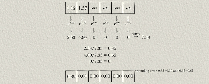
And in such a way the softmax for each row is calculated, thus calculating the attention matrix

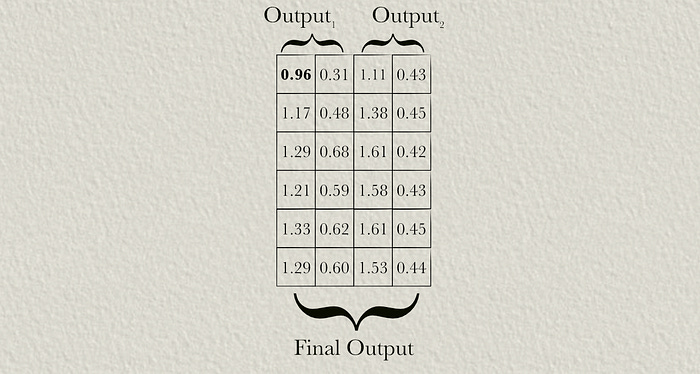
Step 8: Calculating the Output of the Attention Head

Now that we’ve calculated the attention matrix, we can multiply it by the value matrix to construct the output of the attention head.

Step 9: Concatenating the Output

Both attention heads create a distinct output, which are concatenated together to produce the final output of multi headed self attention.

Conclusion

And that’s it. In this article we covered the major steps to computing the output of MHSA:

1. defining the input

2. defining the learnable parameters of the mechanism

3. calculating the Query, Key, and Value

4. diving into multiple heads

5. calculating the Z matrix

6. masking

7. calculating the attention matrix

8. calculating the output of the attention head

9. concatenating the output

If you’re interested in understanding the theory, check out the IAEE article:

---

---

Join IAEE

At IAEE you can find:

• Long form content, like the article you just read

• Thought pieces, based on my experience as a data scientist, engineering director, and entrepreneur

• A discord community focused on learning AI

• Lectures, by me, every week