
What Are Gradients, and Why Do They Explode?
By reading this post you will have a firm understanding of the most important concept in deep learning


Gradients are arguably the most important fundamental concept in machine learning. In this post we will explore the concept of gradients, what makes them vanish and explode, and how to rein them in.
Who is this useful for? Beginning to Intermediate data scientists. I’ll include some math references which may be useful for more advanced readers.
What will you get from this post? An in depth conceptual understanding of gradients, how they relate to machine learning, the issues that come from gradients, and approaches used to mitigate those issues.
What is a Gradient?
Imagine you have some surface with hills and valleys. This surface is defined by some multidimensional function (a function with multiple inputs).
"""
Making a 3d surface with hills and vallys, for demonstrative purposes
"""

import matplotlib.pyplot as plt
from matplotlib import cm
from matplotlib.ticker import LinearLocator
import numpy as np

#creating wide figure
fig, ax = plt.subplots(subplot_kw={"projection": "3d"})

# Make data.
X = np.arange(-5, 5, 0.25)
Y = np.arange(-5, 5, 0.25)
X, Y = np.meshgrid(X, Y)
R = np.sqrt(X**2 + Y**2)
Z = 0.2*np.sin(X+Y + R) - 1*np.sin(X/2)

# Plot the surface.
surf = ax.plot_surface(X, Y, Z, cmap=cm.viridis,
                       linewidth=0, antialiased=False)

plt.show()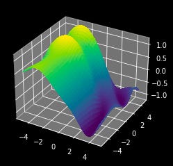
A gradient tells you, for any given point on the surface, both the direction to get to a higher point on the surface, as well as how steep the surface is at that point.
Because this is a 3d surface (the inputs are x and y, and the output is z) we can compute a simplified version of the gradient by computing the slope of a given point along the X axis and the Y axis.
"""
Calculating a simplified gradient using slopes along the X and Y direction
"""

def computeZ(x,y):
    """
    calculates any point on the surface
    """
    r = np.sqrt(x**2 + y**2)
    z = 0.2*np.sin(x+y + r) - 1*np.sin(x/2)

    return z

def plot_pseudo_gradient(x,y):
    """
    Calculates an approximation of the gradient using slope calculations
    of neighboring points offset by a small dx and dy.
    """

    #computing value at point
    z = computeZ(x,y)

    #defining some small distance to traverse
    dx = 0.9
    dy = 0.9

    #getting the change in Z as a result of the change in X and Y
    dzx = (computeZ(x+dx,y) - computeZ(x,y))
    dzy = (computeZ(x,y+dy) - computeZ(x,y))

    #calculating the slope along the x and y axis.
    #these together tell you the direction of increase
    #and the slope of the current point, so these together
    #are the actual pseudo gradient
    slope_x = dzx/dx
    slope_y = dzy/dy

    #to scale the vectors for visability
    scale = 7

    #calculating the value at the end of the pseudo gradient
    #so I can draw a tangent line along the surface in the direction
    #of the gradient
    dz = computeZ(x+slope_x*scale,y+slope_y*scale)

    xs = [x, x+slope_x* scale]
    ys = [y, y+slope_y* scale]
    zs = [z, z+dz]

    #plotting the actual gradient
    ax.plot([xs[0], xs[1]],
            [ys[0],ys[1]],
            [zs[0],zs[0]], 'b')

    #plotting the tangent line
    ax.plot(xs, ys, zs, 'r')

    #plotting vector components of the tangent line
    ax.plot([xs[0],xs[1],xs[1],xs[1]],
            [ys[0],ys[0],ys[1],ys[1]],
            [zs[0],zs[0],zs[0],zs[1]], '--k')

    ax.scatter([x],[y],[z], marker='x', c=['k'])

#creating a figure
fig, ax = plt.subplots(subplot_kw={"projection": "3d"})
ax.computed_zorder=False #unfortunatly, zorder has pervasive bugs in 3d plots

# Plot the surface.
surf.set_zorder(1)
surf = ax.plot_surface(X, Y, Z, cmap=cm.viridis, linewidth=0, antialiased=False, alpha=0.2)
surf.set_zorder(1)

#plotting the pseudo gradient at x=0 and y=0
plot_pseudo_gradient(0,0)

#rendering
plt.show()

#for later use in traversal with the gradient
return slope_x, slope_y
So, to summarize that conceptually, the gradient computes the direction of greatest increase, and how steep that increase is, by calculating the slope of the output relative to all inputs of a function.
Actual Gradients
In the previous example I computed what I referred to as a “simplified gradient”. I calculated the slope of z relative to a small change in x and a small change in y.

In reality, gradients are calculated using a partial derivative, meaning it’s a derivative of the function with respect to a single variable (x or y). If you’re unfamiliar with calculus you can watch a quick video on derivatives and another on partial derivatives to get up to speed on the math. However, regardless of the math, the concepts of the simplified gradient and actual gradient are identical.
Gradients in a Simple Model
When researching machine learning you’ll find differentiability everywhere; differentiable loss functions, differentiable activation functions, etc. etc. The reason for this is, if everything's differentiable, you can quickly calculate the gradient (the direction in which you need to adjust inputs to functions to get a better output).
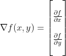
For example, suppose we have a machine learning model with two parameters, x and y. We also have a function that tells us how well those parameters fit the model to a set of data. We can use gradients to try to find the best model parameters by taking a series of steps in the direction the gradient.
"""
Using Gradients to iteratively search for the maximum of the surface
"""

#creating a figure
fig, ax = plt.subplots(subplot_kw={"projection": "3d"})
ax.computed_zorder=False #unfortunatly, zorder has pervasive bugs in 3d plots

# Plot the surface.
surf.set_zorder(1)
surf = ax.plot_surface(X, Y, Z, cmap=cm.viridis, linewidth=0, antialiased=False, alpha=0.3)
surf.set_zorder(1)

#iteratively following the gradient
x,y = 0,0
for _ in range(10):
    dx,dy = plot_pseudo_gradient(x,y)
    x,y = x+dx, y+dy

#rendering
plt.show()

#printing result
print("ideal parameters: x={}, y={}".format(x,y))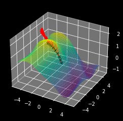
When people talk about training they sometimes refer to a “loss landscape”. When you turn a problem into a machine learning problem, you are essentially creating a landscape of parameters which perform better, or worse than others. You define what is good, and what is bad (the loss function) and a complex function with a set of differentiable parameters which can be adjusted to solve the problem (the machine learning model). These two, together, create a theoretical loss landscape, which one traverses through gradient descent (model training). But What is Gradient Descent?
A gradient, mathematically, is used to point towards a greater value in a function. In machine learning we usually optimize to reduce the error rate, so we want our loss function (how many errors we make) to be smaller, not bigger. The math is virtually identical though; you just turn a few +’s into -’s
"""
reworking the previous example to find the minumum with gradient descent
"""

fig, ax = plt.subplots(subplot_kw={"projection": "3d"})
ax.computed_zorder=False

surf.set_zorder(1)
surf = ax.plot_surface(X, Y, Z, cmap=cm.viridis, linewidth=0, antialiased=False, alpha=0.3)
surf.set_zorder(1)

x,y = 0,0
for _ in range(10):
    dx,dy = plot_pseudo_gradient(x,y)
    x,y = x-dx, y-dy #<----------- this is the only part that changed

plt.show()

print("ideal parameters: x={}, y={}".format(x,y))
What Are Exploding and Vanishing Gradients?
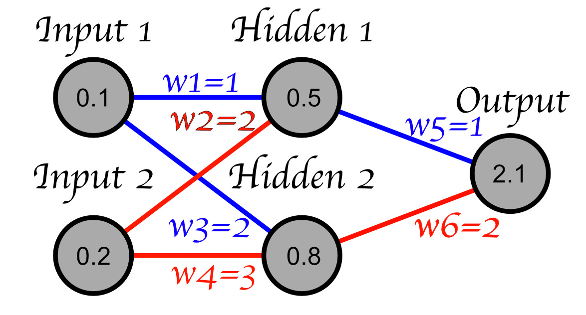
First, let’s look at a simplified neural network. We’re going to ignore the activation functions and bias and just think of a neural network as a series of weights. Under this set of simplifications, a neural network looks like this
The issue of exploding and vanishing gradients comes into play when we have deeper neural networks. Imagine a network with several more layers multiplying and adding, multiplying and adding, etc.
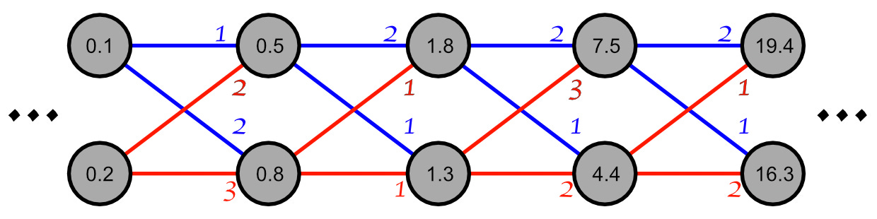
As you can see, the values quickly become large when you consistently multiply by numbers which are larger than 1. With weights which are less than 1 the values would quickly shrink as they are multiplied by smaller and smaller values.
We can see that the values within the network can get large or small quickly depending on the weights within the model, but we can also imagine the values listed within each perceptron as a change, rather than a value.
The punchline is this: Repeated multiplication can cause the rate of change (gradient) to get really big if the weights are larger than one, or really small if the weights are less than 1. In other words, the gradients can explode or vanish.
Why Are Exploding and Vanishing Gradients Bad?
Big gradients, small gradients, so what?
Small gradients move slowly, and have a tendency to get stuck in shallow local minima. As a result, having vanishing gradients can result in a lack of model improvement. On the other hand, exploding gradients move too quickly and can bounce around erratically, leading to an inability for the model to converge on a minima.
"""
Plotting 3 similar landscapes scaled vertically
to have small, moderate, and large gradients
"""

def f(x, scale):
    """
    Function to represent the landscape we are attempting to optimize
    scaling the function vertically will scale the gradients proportionally
    """
    return scale*(0.3*np.sin(x*0.1) +0.5* np.sin(np.cos(x)) + 0.1*np.sin(x*0.3+2) + 4*np.cos(x*0.1) + 6*np.sin(x*0.05))

def f_slope(x, scale):
    """
    Using a pseudo derivative instead of computing the actual derivative
    """
    dx = 0.00001
    slope = (f(x+dx, scale)-f(x, scale))/dx
    return slope

#defining range
X = np.linspace(50,125,10000)

for gradient_scale, color in zip([1,10,100], ['r', 'y', 'b']):
    #computing landscape
    Y = np.array(list(map(f, X, [gradient_scale]*len(X))))

    point = 58
    explored_x = []
    explored_y = []
    for _ in range(20):

        #marking point as explored
        explored_x.append(point)
        explored_y.append(f(point,gradient_scale))

        #traversing along gradient
        point = point-f_slope(point, gradient_scale)

    #plotting landscape
    plt.plot(X,Y)
    #plotting traversal
    plt.plot(explored_x, explored_y, 'x-'+color)
    #rendering
    plt.show()
This problem becomes even more pervasive when you consider that not only does the larger model have a gradient, each individual perceptron has a gradient as well. this means that different perceptrons within a network can have very different gradients. In theory, a model can have vanishing and exploding gradients at the same time in different parts of the model.
How Do We Fix Exploding and Vanishing Gradients?
1) Adjust the Learning Rate
The learning rate gets multiplied by the gradient to control how far of a step gets taken along the gradient for each iteration. Smaller learning rates result in small steps, while large learning rates result in larger steps (I did something roughly equivalent in the previous example). This can be useful to a point, but the issue with vanishing and exploding gradients is that the gradients change throughout the model (some perceptrons have small changes, and others have large changes). So, while learning rate is a critical hyperparameter, it’s not usually considered as an approach for dealing with vanishing and exploding gradients specifically.
2) Change Activation Functions
For a variety of reasons, perceptrons don’t just multiply their inputs by some weight, add the results together, and spit out an output. Virtually all networks pass the result of this operation through a function called an activation function. Activation functions are all differentiable, and thus have a variety of characteristics in effecting the gradients throughout the depth of a network.
4) Change Model Architectures
Simply having a shorter network can help. However, if that’s not an option, several network architectures were designed specifically to handle this problem. LSTMs were designed to be more robust than classical RNNs at dealing with exploding gradients, residual and skip connections are also designed to aid in solving this phenomenon.
5) Use Batch Normalization
Batch normalization is a mainstay regularization strategy in machine learning. Instead of updating a model parameters by a single gradient, you update parameters by using the average gradient from a batch of examples.
6) Gradient Clipping
You can just set a maximum allowable threshold for a gradient. If the gradient is larger than that, just set the magnitude of the gradient to be the threshold.
7) Use Weight Regularizers
L1 and L2 regularization are used to penalize models for having high weight values. Adding this form of regularization can reduce exploding gradients.
8) Truncate Context Windows
Whether you’re using a recurrent network, or some other network which employs a context window, reducing the size of that window can help minimize compounding gradient issues.
Conclusion
And that’s it! In this post we learned a bit about gradients and the math behind them. We learned you can use gradients to go up or down surfaces within some dimensional space, and how that’s used to optimize machine learning models. We learned that, as a model grows in size, the gradients can explode to large numbers, or vanish to very tiny numbers, both of which can ruin the models ability to learn. We also went through a list of approaches for correcting vanishing and exploding gradients.
Follow For More!
In a future post I’ll be describing several landmark papers in the ML space, with an emphasis on practical and intuitive explanations. I also have posts on not-so commonly discussed ML concepts.
I would be thrilled to answer any questions or thoughts you might have about the article. An article is one thing, but an article combined with thoughts, ideas, and considerations holds much more educational power!