
Apache Spark — Intuitively and Exhaustively Explained
An in depth exploration of modern, large scale data processing


In this article we’ll discuss Apache Spark, a popular computing system designed for modern, large scale data processing.
Netflix, Uber, Facebook, JPMorgan Chase, Amazon, and many more major companies use Spark to do a huge number of critical operations on a daily basis. In this article we’ll explore why Spark is useful, and how it works.
Who is this useful for? Anyone interested in building cutting edge data processing pipelines at-scale
How advanced is this post? This article is designed to be a first principles conceptual breakdown of spark, and is accessible to readers of all levels.
Prerequisites: None, though Python experience is recommended in understanding the implementation section. Experience in SQL, Pandas, and Polars is also helpful.


A Core Problem
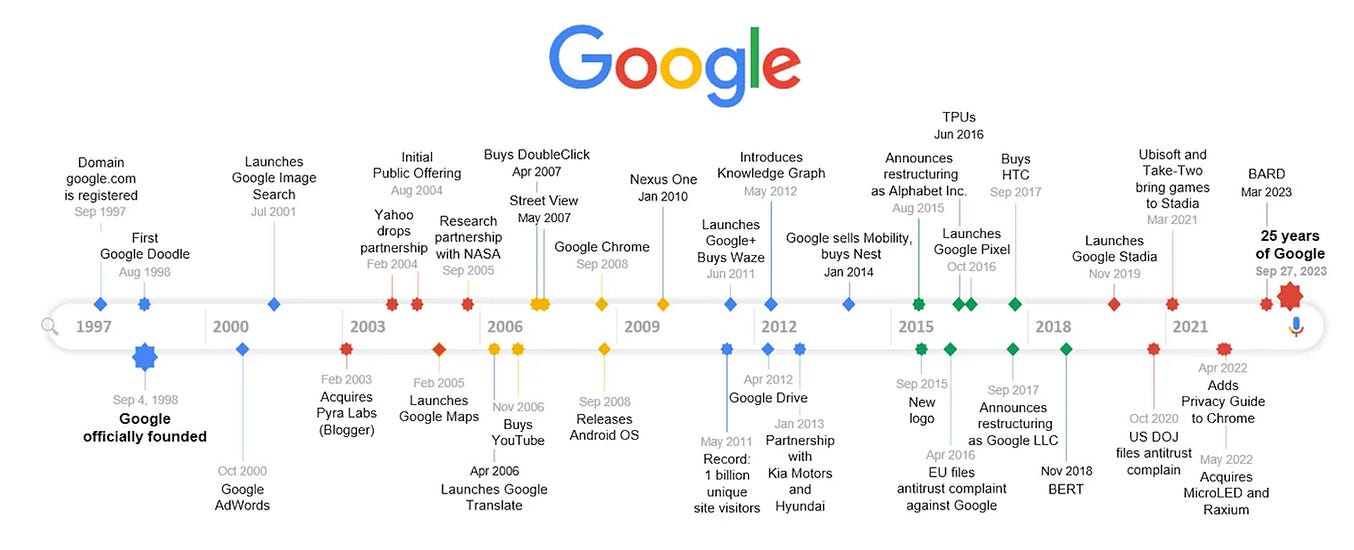
In the early 2000s, Google was on the verge of an absurd amount of growth.
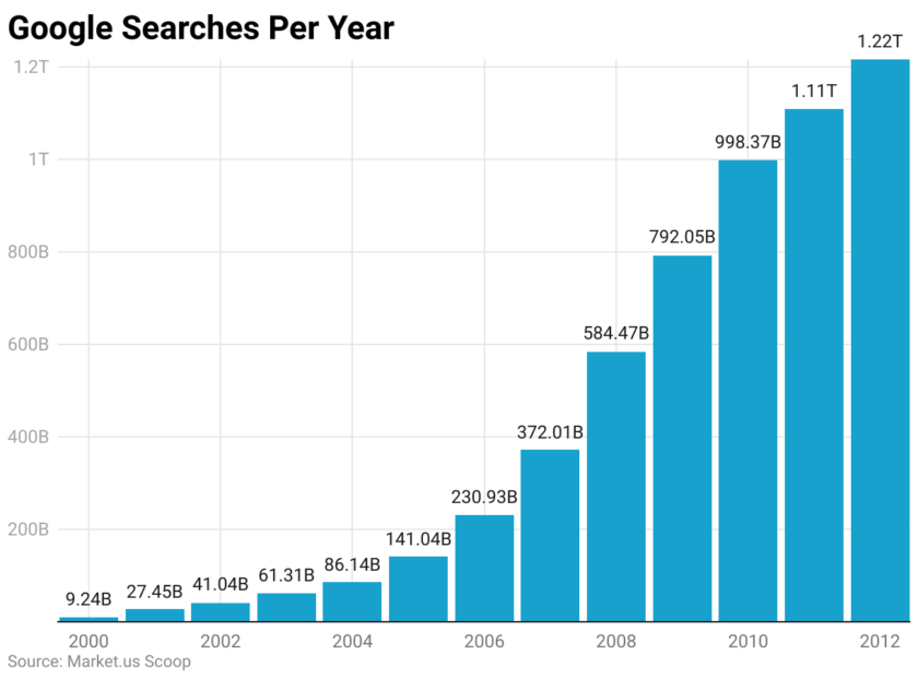
And, on top of that, they were gearing up to release a huge number of what would later become wildly successful products.
These required massive computational resources; think creating search indexes, sorting, data mining, machine learning, and doing statistical analysis. On the volume of data Google was working with, many of their operations couldn’t be done on a single machine. Instead, many computers had to work together to tackle these problems.
At the time, getting work like this done was un-standardized. Google had a variety of technologies for distributed data management, but it was up to very experienced developers to stitch these together when building any new, major parallel operation.
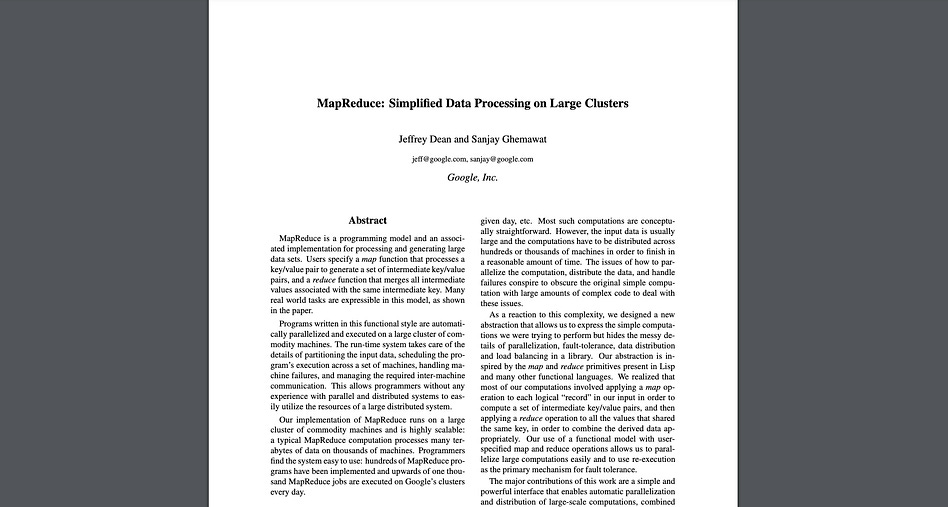
Enter MapReduce, the predecessor to Spark.
MapReduce
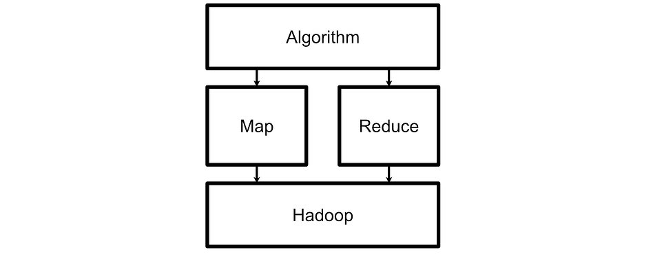
Engineers at Google realized that the majority of their bespoke parallelization code was doing the same two fundamental operations:
Map: Transforming an input into some output given a function
Reduce: Accumulate results together.
For example:
If you wanted to count all the word occurrences in a large document (how often each word is used), you could map all of the pages into a word count, then take all of the word counts for all pages and reduce them to a single word count.
If you wanted to calculate how often certain websites are linked, you can map each website to a list of links then reduce that to a count across all websites.
If you wanted to calculate the average luminosity of all videos on a social media platform, you can map each video into an average luminosity across the video, then reduce that across all videos.
Because so many different types of large scale, common operations could be easily conceptualized with mapping and reduction, Google decided to make a framework specifically for these operations, called MapReduce.
The high level workflow of MapReduce is defined with three key things:
The input data, and how it can be logically divided.
A mapping function, that can work on an individual piece of data.
A reduction function, that can take many different mapped values and convert them into an output representation.
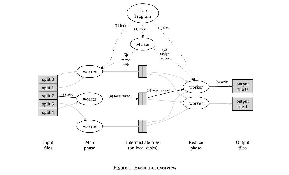
There are more details under the hood. For instance, MapReduce uses a concept of shuffling to randomly distribute load, and key/value pairs to control which data is allowed to be reduced, but these specifics are out of scope for this article. What’s important to know, though, is how MapReduce functions in essence: it splits data up into bite sized operations so that different computers can work on the problem in parallel, and it does that in a standardized way that allows one to leverage a large cluster of computers without needing to code up all the low level parallelization.
MapReduce was a dominant paradigm for a long time. It allowed individual developers to implement solutions that previously required large and expensive multi-disciplinary teams. Also, the standardization of so many different tasks into a single framework allowed the industry to standardize on a universal set of tooling. “Apache Hadoop” was an incredibly popular framework for doing MapReduce at scale, and allowed companies to standardize their tooling around how Hadoop implemented MapReduce.
To make MapReduce work at scale, Hadoop implemented a bunch of critical components which work in conjunction with MapReduce:
YARN (Yet Another Resource Negotiator): manages cluster resources (like how CPUs and memory get allocated throughout a cluster) and task scheduling.
HDFS (Hadoop Distributed File System): Designed to store large datasets across many systems, with redundant stores for fault tolerance.
A bunch of tools for data management, compatability with many file formats, search tools, and other fun stuff.
This was a paradigm shift for large scale computing. Before Hadoop, large scale parallel jobs were largely bespoke. Now, standardized tools could be plugged into a standardized system, allowing for unprecedented interoperability at scale.
The Issue With Hadoop
Hadoop is still used at a large number of companies, and for good reason; it has a mature ecosystem which is well integrated with the needs of many large scale companies that need large scale data processing. However, if you pull a data engineer to the side in 2025 and ask them what tool is worth learning, most of them will say Spark is more important than Hadoop.
The main problem with Hadoop is the times it was designed in. Hadoop hit the scene in 2006 when cheap harddrives was the norm, RAM was expensive, and machines failed all the time. The name of the game was fault tolerance over speed, so Hadoop spends a lot of time saving data to and reading from disk.
In 2012, when spark was released, this paradigm was starting to feel dated. RAM was much more plentiful, networks were faster and more reliable, and more robust processing tasks were in higher demand. Some of the core design paradigms which made Hadoop a success were losing relevance.
Enter Spark
If you go to the main site for Apache Spark, it defines the project as:
Apache Spark™ is a multi-language engine for executing data engineering, data science, and machine learning on single-node machines or clusters.
The Wikipedia page says:
Spark provides an interface for programming clusters with implicit data parallelism and fault tolerance
And the PySpark PyPI page describes Spark as
Spark is a unified analytics engine for large-scale data processing. It provides high-level APIs in Scala, Java, Python, and R, and an optimized engine that supports general computation graphs for data analysis. It also supports a rich set of higher-level tools including Spark SQL for SQL and DataFrames, pandas API on Spark for pandas workloads, MLlib for machine learning, GraphX for graph processing, and Structured Streaming for stream processing.
In Hadoop, you had an engine that just did MapReduce. Spark, in contrast, is more general purpose, has more complex functionality, and is thus harder to define. Spark is inspired by Hadoop, but there are some fundamental differences in their core design principles which make them fundamentally different.
Hadoop expects the developer to define two major tools; map and reduce. Once you implement those tools, Hadoop applies them to your data.
Spark, on the other hand, employs an “execution engine” paradigm. Spark exposes a library of tools which you can choose to employ. These are defined as “transformations” and “actions” which we’ll discuss in future sections.
Spark has tools for map and reduce, which allows Spark to emulate the MapReduce functionality of Hadoop, but the Spark execution engine also has functionality for filtering, sampling, grouping, counting, and iterating, allowing Spark to execute much more complex operations.
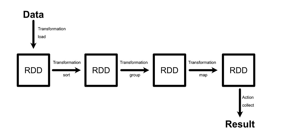
In Hadoop you define two rigidly constrained tools to be broadcast over the cluster. In Spark, you can use a range of more complex pre-defined tools to do much more flexible and sophisticated tasks. To support this more complex general functionality, Spark employs a computational graph which we’ll also explore later.
Another major difference between Spark and Hadoop is that Spark employs an in-memory first design paradigm. Instead of reading and writing to storage, like what Hadoop usually does, Spark tries to keep as much data in-memory as possible, and only relies on storage to drive as a fallback. This makes Spark significantly faster than Hadoop in many applications, and enables real-time analysis of very, very large datasets.
That’s the thousand yard view of Spark. It’s like Hadoop, but it’s more flexible and faster. Let’s dig into some of the core components of spark that make it tick.
Resilient Distributed Datasets (RDDs) and Lazy Evaluation
The “Resilient Distributed Dataset”(RDD) is one of the most fundamental ideas in Spark. RDDs represent distributed collections of data and define what operations should be computed to transform that data across a cluster. They don’t hold the data themselves — instead, they record where the data came from and what transformations should be applied. We’ll cover this more in depth later, for now you can think of RDDs as a record of how data changes throughout a data processing pipeline.
There are four defining properties of RDDs that I think are fundamental to understand when getting into Spark:
Immutable: Once you make an RDD, you can’t change it. If you want to change the data, you have to make a new RDD.
Distributed: RDDs can be stored in a distributed manner across many nodes (computers) within a cluster.
Lazily Evaluated: RDDs don’t hold data per-se, they keep track of where data comes from and what operations have been applied to that data.
Partition-Oriented: RDDs aren’t designed to work on a particular type of data. Rather, they work on partitions of data. You can have text files, images, audio, whatever. RDDs don’t care, they just care if you can sub-divide the data. RDDs manage those subdivisions.
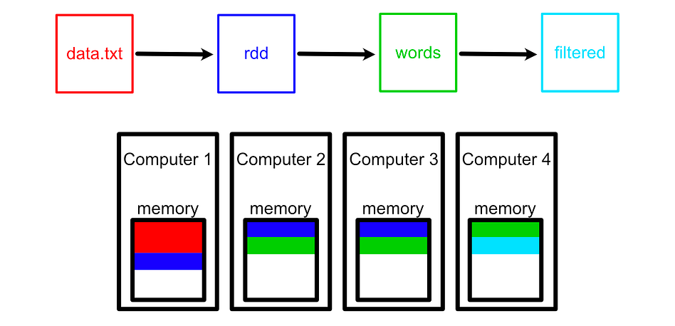
Take, for example, the following PySpark code (PySpark being a way to interface with Spark via Python).
rdd = spark.textFile(”hdfs:///data.txt”)
words = rdd.flatMap(lambda line: line.split())
filtered = words.filter(lambda w: w != “the”)
here, rdd, words, and filter are all RDDs which, when linked together, define a computational graph.
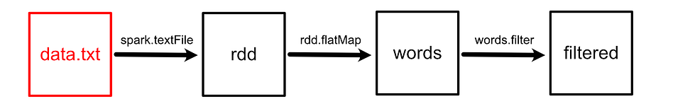
When applying the flatMap operation to rdd, we don’t modify rdd, but rather create a new RDD called words. rdd still exists as an immutable record. Each of these three RDDs are resilient and distributed, meaning they can be referencing data across various different computers.
These computations are not executed by default. Rather, they’re only executed when triggered, for instance, by calling collect on the last RDD.
result = filtered.collect()This triggers Spark to actually execute the computations in the directed graph and provides the final result. This is called lazy evaluation, and it has some compelling benefits which we’ll describe later in the article.
So, Spark uses data divided up into partitions to do large scale processing, and encodes operations applied to those partitions as a chain of RDDs which will be executed when triggered. Before we get into the weeds of building pipelines with Spark, let’s unpack how we can set up spark in the first place.
Setting up Contexts and Sessions in PySpark
Luckily for us, Google Colab already has PySpark installed with all the necessary dependencies and configuration setup. All we have to do is create a spark session. This will allow us to play around with the basics of Spark. If you want to see the full notebook, you can check it out here.
import pyspark

from pyspark.sql import DataFrame, SparkSession
from typing import List
import pyspark.sql.types as T
import pyspark.sql.functions as F

spark= SparkSession \
       .builder \
       .appName(”sparkApp”) \
       .master(”local[*]”) \
       .getOrCreate()

spark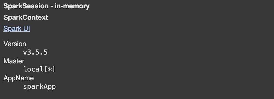
Here, we’re creating both a “context” and a “session”.
A context in spark defines the cluster we’ll be connecting to. .master(“local[*]”) defines that we want to run spark locally, so we’re not connecting to some external cluster to do massively parallelized computation, we’re just using the colab instance we’re running. [*] defines that we want to use all available CPU cores. We could also specify [1], [2], or some other number to constrain spark to a certain number of cores.
Of course, the power of spark is in its ability to connect to an external cluster. You can use something like Amazon EMR, Google Dataproc, or DataBricks to spool up a cluster, then you would simply connect to it by pointing to the IP and port like so.
spark = SparkSession.builder \
    .appName(”ClusterApp”) \
    .master(”spark://192.168.1.10:7077”) \
    .getOrCreate()
So, a spark context defines the compute resources you’re connecting to. In PySpark, each process can only be connected to a single context, so if you want to establish two separate contexts you’ll need to, for instance, run two seperate python scripts.
Within a single context, though, you can have numerous “sessions”. A session in Spark is an isolated scope of data and functionality which is defined within our context. So, if we had a single spark context which was connected to a large spark compute cluster, we could create and manage several sessions within that context all from a single Python script.
When we call getOrCreate we’re telling spark that we want to either create a new session or connect to an existing session. We can then create multiple other sessions which are isolated.
Here’s an example of creating two different spark sessions with different data.
from pyspark.sql import SparkSession

# First, we initialize a SparkSession and SparkContext
spark1 = SparkSession.builder.appName(”sparkApp”).getOrCreate()

# Create a DataFrame and a temporary view in spark1
df1 = spark1.createDataFrame([(1, “Alice”), (2, “Bob”)], [”id”, “name”])
df1.createOrReplaceTempView(”people”)

# Run SQL in spark1
print(”Session 1:”)
spark1.sql(”SELECT * FROM people”).show()

# Now create a separate session
spark2 = spark1.newSession()

# Session 2 does NOT see the temp view from session 1
print(”Session 2 (before creating view):”)
try:
    spark2.sql(”SELECT * FROM people”).show()
except Exception as e:
    print(”Error:”, e)

# Create a separate view in session 2
df2 = spark2.createDataFrame([(3, “Charlie”)], [”id”, “name”])
df2.createOrReplaceTempView(”people”)

print(”Session 2 (after creating its own view):”)
spark2.sql(”SELECT * FROM people”).show()

print(”Back to Session 1:”)
spark1.sql(”SELECT * FROM people”).show()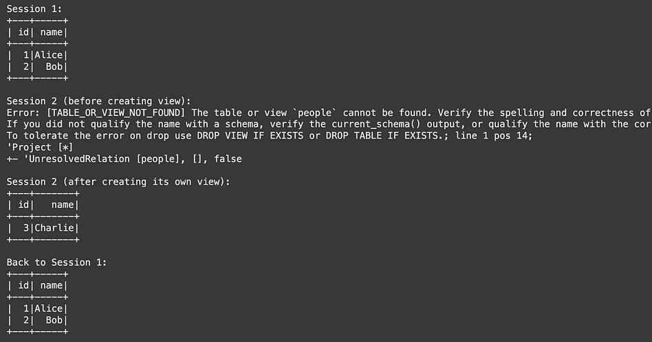
Without getting into the weeds of exactly what this code is doing, you can see that each session contains separate data, but if we print out the high level sessions we can see that they both belong to the same context (via the AppName).
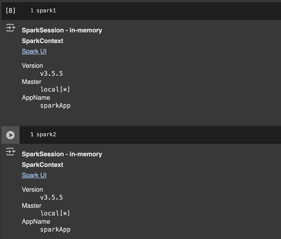
So, the sessions have different data which is logically isolated, but that data occupies the same physical hardware.
One quirk, which I mentioned before, is that there can only be one context per python process. Since we already created a context with the name sparkApp, and it already has a session associate with it, if we try to create new spark contexts they’ll end up defaulting to our existing session.
spark1 = SparkSession.builder.appName(”AppOne”).getOrCreate()
spark2 = SparkSession.builder.appName(”AppTwo”).getOrCreate()

print(spark1 is spark2)  # True — same session
print(spark2.sparkContext.appName)  # “AppOne”
This can be a bit counterintuitive if you don’t understand the underlying nature of contexts and sessions. You might think you’re building a unique session by assigning a different appName, but spark only allows a single context per process so it simply loads up our old sparkApp.
Creating an RDD and Evaluating Computational Graphs
One of the most fundamental concepts within spark is the “Resiliant Distributed Dataset” (RDD). RDDs are how Spark can take a single source of data and distribute it over many seperate computers to parallelize computation.
There are many ways to create RDDs. Here, we’ll create a simple RDD from scratch using a Python List.
from pyspark.sql import SparkSession

# ---- Setup ----
spark = SparkSession.builder.appName(”RDD Demo”).getOrCreate()
sc = spark.sparkContext

# ---- Create RDDs ----
numbers = sc.parallelize([1, 2, 3, 4, 5])
This creates an RDD called numbers , which is automatically divided into some number of partitions based on the cluster we’re working on. We could do some operation to this data, like add 10 to each number.
# ---- Transformation: add 10 to each number ----
added = numbers.map(lambda x: x + 10)
Here the map function takes x, one of the numbers in our original list, and replaces it with x+10, effectively adding 10 to each element in the list. If we print the results of added, however, we don’t get a list of numbers but rather a reference to an RDD.
print(added)
This RDD is a placeholder for what we would get if we did add 10 to each value. Recall that Spark is evaluated lazily, meaning we can line up all the calculations we want it to do, but it wont actually do those calculations untill we tell it to. We can do that with the collect function.
# ---- Action: collect results back to the driver ----
result = added.collect()

print(”Original numbers:”, numbers.collect())
print(”After adding 10:”, result)
The whole point of an RDD is that it allows us to manage how data is distributed across various different machines. We can actually inspect the partitions that get created via the following:
numbers = sc.parallelize([1, 2, 3, 4, 5])
print(numbers.glom().collect())
The glom transformation allows you to view the content of each partition as a python list, then we can call collect to actually run that function and view the result. As you can see, 8 partitions were created, as there are 8 cores in my machine. The content of the list is distributed within that list of available partitions. We could also reduce the number of partitions
#the 2 means we want the data to be parallelized across 2 partitions
numbers = sc.parallelize([1, 2, 3, 4, 5], 2)
print(numbers.glom().collect())
or add more data that could fill out our default of 8 partitions.
numbers = sc.parallelize([1, 2, 3, 4, 5, 6, 7, 8, 9, 10, 11, 12, 13, 14, 15])
print(numbers.glom().collect())
We can do several operations on this data simultaniously. For instance, imagine we wanted to print out the following lists:
a list of input numbers
a list of all those numbers squared
a list of all of the squares that are even numbers
a sum of all of the numbers
a sum of all of the even squares
We can do that with the following code:
from pyspark.sql import SparkSession

# ---- Setup ----
spark = SparkSession.builder.appName(”RDD Demo”).getOrCreate()
sc = spark.sparkContext

# ---- Create RDDs ----
numbers = sc.parallelize([1, 2, 3, 4, 5])

# ---- Transformations ----
squared = numbers.map(lambda x: x * x)
even_squares = squared.filter(lambda x: x % 2 == 0)

# ---- Reduce ----
total = numbers.reduce(lambda a, b: a + b)
total_even_squares = even_squares.reduce(lambda a, b: a + b)

# ---- Printing ----
print(”Original numbers:”, numbers.collect())
print(”Squared:”, squared.collect())
print(”Even squares:”, even_squares.collect())
print(”Sum of numbers:”, total)
print(”Sum of even squares:”, total_even_squares)

spark.stop()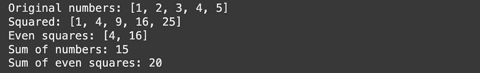
There’s some new concepts going on in this code that I’d like to break down. First of all, we’re creating an RDD consisting of a list of numbers, same as before.
# ---- Setup ----
spark = SparkSession.builder.appName(”RDD Demo”).getOrCreate()
sc = spark.sparkContext

# ---- Create RDDs ----
numbers = sc.parallelize([1, 2, 3, 4, 5])
We’re then applying transformations to the data, in the form of a mapping function.
# ---- Transformations ----
squared = numbers.map(lambda x: x * x)
even_squares = squared.filter(lambda x: x % 2 == 0)
There are many other transformations that can be performed in spark. Sorting, inner and outer joins, sampling, and filtering to name a few. You can chain many transformations together, and Spark will construct an execution graph of how the different operations inter-relate with one another.
If you want to actually trigger the computational graph, you need to call an “Action”. collect is one such action. It triggers the computational graph and returns the result as a list. reduce is another action that, instead of returning all results as a list, combines all results into a single value based on a function.
# ---- Reduce ----
total = numbers.reduce(lambda a, b: a + b)
total_even_squares = even_squares.reduce(lambda a, b: a + b)
recall that spark groups data into partitions

Each partition might have multiple values it’s working on. the reduce function first combines all pairs of values in a single partition into a single value, then combines all pairs of values across partitions into a single value. Thus by using the reduction function (lambda a, b: a + b), we’re effectively telling spark to add up all values across all partitions.
# ---- Printing ----
print(”Original numbers:”, numbers.collect())
print(”Squared:”, squared.collect())
print(”Even squares:”, even_squares.collect())
print(”Sum of numbers:”, total)
print(”Sum of even squares:”, total_even_squares)
To actually print out our output, some RDDs need to have collect called on them, because they were not evaluated. However, total and total_eve_squares are not RDDs, but actual values. We triggered them to be evaluated when we called reduce, which is an action and not a transformation.
So, in simple words:
you can chain actions together, to create a chain of RDDs.
when you call an action, like
collectorreduce, it actually triggers that chain of transformations and returns a result.
There’s an important note in this example; it’s inefficiently implemented. We calculate squares, filter those into even squares, then calculate the sum of all of the even squares. One might expect the computation to look something like this:
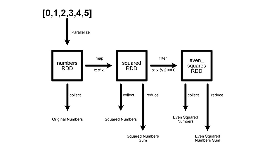
however, in actuality, we’re defining five different computational graphs that are executed separately for each action we undertake.
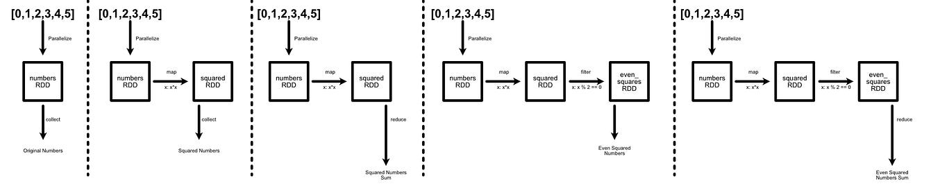
This means we’re wastefully re-computing the same thing over and over again. Not a big deal if you’re processing a list of five numbers, huge deal if you’re processing petabytes of data. One way one might alleviate this issue is to use caching.
from pyspark.sql import SparkSession

# ---- Setup ----
spark = SparkSession.builder.appName(”RDD Caching Demo”).getOrCreate()
sc = spark.sparkContext

# ---- Create RDD ----
numbers = sc.parallelize(range(1, 11))  # 1 to 10

# ---- Transformations ----
squared = numbers.map(lambda x: x * x)
even_squares = squared.filter(lambda x: x % 2 == 0)

# -------------------------------
# Without caching: Spark recomputes each time
# -------------------------------
print(”=== WITHOUT CACHING ===”)
print(”Squared:”, squared.collect())          # triggers a Spark job
print(”Even squares:”, even_squares.collect()) # recomputes from numbers → squared → even_squares
print(”Sum of even squares:”, even_squares.reduce(lambda a, b: a + b))  # recomputes again

# -------------------------------
# With caching: Spark computes once and reuses results
# -------------------------------
squared_cached = numbers.map(lambda x: x * x).cache()
even_squares_cached = squared_cached.filter(lambda x: x % 2 == 0).cache()

print(”\n=== WITH CACHING ===”)
print(”Squared (cached):”, squared_cached.collect())            # first action → computed & cached
print(”Even squares (cached):”, even_squares_cached.collect())  # reused from cache, and result stored to cache
print(”Sum of even squares (cached):”, even_squares_cached.reduce(lambda a, b: a + b))  # reused cache

# ---- Clean up ----
spark.stop()
Here, the same spark code is implemented twice. First without caching (exactly as was done previously), and second with caching. If an RDD with caching is triggered for execution, it does the following:
If the RDD hadn’t been executed previously, do all proceeding computations, store the result, and return the result.
If the RDD had been executed previously, and a value is stored, don’t do proceeding operations and simply return the stored value.
This allows us to effectively re-use computations.
Even without proceeding in this article, you’ve unlocked a massive tool for doing large scale parallelized work. If you can turn your data into a partitioned RDD, you can specify transformations, actions, and caching to do massively parallelized work across large datasets by using the power of a cluster of computers. For instance, this code snippet applies similar concepts of parallelization we previously explored, but applies it to audio processing.
import matplotlib.pyplot as plt
import librosa

spark = SparkSession.builder.appName(”Audio FFT DAG Demo”).getOrCreate()
sc = spark.sparkContext

audio_files = [os.path.join(”test_audio”, f) for f in os.listdir(”test_audio”)]
rdd = sc.parallelize(audio_files)

# ==========================================
# Step 3. Define DAG transformations
# ==========================================
def load_audio(path, sr=22050):
    import librosa  # This is happening inside a worker, so we need to import
    y, sr = librosa.load(path, sr=sr)
    return (path, y, sr)

def compute_fft(item):
    import numpy as np  # This is happening inside a worker, so we need to import
    fname, y, sr = item
    fft_vals = np.fft.fft(y)
    return (fname, y, sr, fft_vals)

def compute_ifft(item):
    import numpy as np  # This is happening inside a worker, so we need to import
    fname, y, sr, fft_vals = item
    y_reconstructed = np.fft.ifft(fft_vals).real
    return (fname, y, sr, fft_vals, y_reconstructed)

# DAG
audio_rdd = rdd.map(load_audio).cache()
fft_rdd = audio_rdd.map(compute_fft).cache()
ifft_rdd = fft_rdd.map(compute_ifft).cache()

# ==========================================
# Step 4. Execute DAG + Collect
# ==========================================
results = ifft_rdd.collect()

# ==========================================
# Step 5. Plot results
# ==========================================
for fname, y, sr, fft_vals, y_reconstructed in results:
    # --- 1. Original waveform ---
    plt.figure(figsize=(3, 0.5))
    librosa.display.waveshow(y, sr=sr)
    plt.title(f”Waveform of {os.path.basename(fname)}”)
    plt.xlabel(”Time (s)”)
    plt.ylabel(”Amplitude”)
    plt.show()

    # --- 2. FFT spectrum ---
    fft_freqs = np.fft.fftfreq(len(fft_vals), 1/sr)
    plt.figure(figsize=(3, 0.5))
    plt.plot(fft_freqs[:len(fft_vals)//2], np.abs(fft_vals)[:len(fft_vals)//2])
    plt.title(f”FFT Spectrum of {os.path.basename(fname)}”)
    plt.xlabel(”Frequency (Hz)”)
    plt.ylabel(”Magnitude”)
    plt.show()

    # --- 3. Reconstructed waveform ---
    plt.figure(figsize=(3, 0.5))
    librosa.display.waveshow(y_reconstructed, sr=sr)
    plt.title(f”Reconstructed Waveform of {os.path.basename(fname)}”)
    plt.xlabel(”Time (s)”)
    plt.ylabel(”Amplitude”)
    plt.show()

# ==========================================
# Step 6. Cleanup
# ==========================================
spark.stop()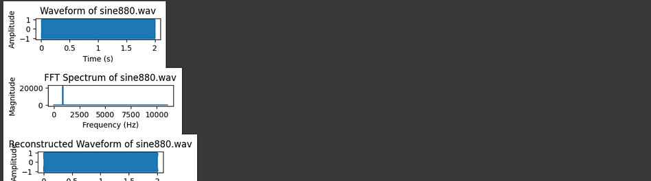
If you’re not familiar with audio processing, don’t worry about it. The point of this code block is to communicate that the general paradigm of RDDs are applicable to a wide range of data types. Here, instead of thinking of an RDD as a list of numbers, I’m thinking of it as a list of file names called rdd. Then, I’m actually loading the data, resulting in audio_rdd. Then I’m doing audio processing techniques to turn audio_rdd into fft_rdd and ifft_rdd, which represent the output of fancy audio processing techniques (You can read more about audio processing here, if you’re interested).
Thus, with spark, doing arbitrary, massively parallelized workloads is as simple as defining a few functions and connecting to a cluster.
Let’s continue our exploration of spark by exploring some of the cool abstractions that are commonly used on top of Spark to make it even easier to use.
Data Frames and SQL
Most data scientists are familiar with dataframes, a la Pandas or Polars. Spark also has a dataframe concept, built on top of RDDs. We can point PySpark to a csv file using the following code:
df = spark.read.csv(’/content/’+csv_file_name, header=True, inferSchema=True)This will create an RDD which I nameddf, which stands for “Data Frame”. If you’re familiar with popular libraries like Pandas or Polars, or even if you’re familiar with Microsoft Excel, you’re familiar with the concept of a data frame. It’s an object that stores data contained in rows and columns.
Because tabular data is so common, Spark allows you to define a dataframe that’s built on top of RDDs, allowing for the parallelized processing of large amounts of row and column based data. We can use all of the same functions you might use in a normal dataframe library, like describe
#Summary stats
df.describe().show()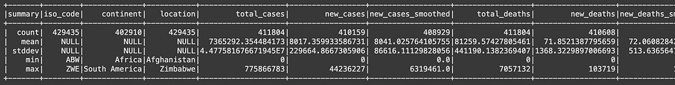
We can do stuff like filtration and ordering
#DataFrame Filtering
df.filter(df.location == “United States”).orderBy(F.desc(”date”)).show()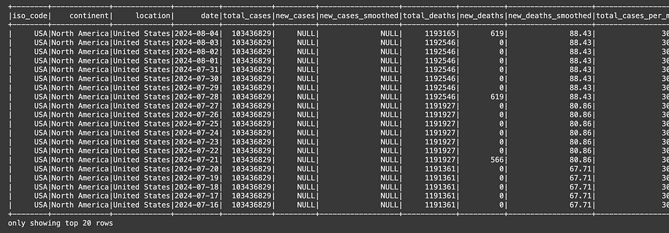
Grouping
#Simple Group by Function
df.groupBy(”location”).sum(”new_cases”).orderBy(F.desc(”sum(new_cases)”)).show(truncate=False)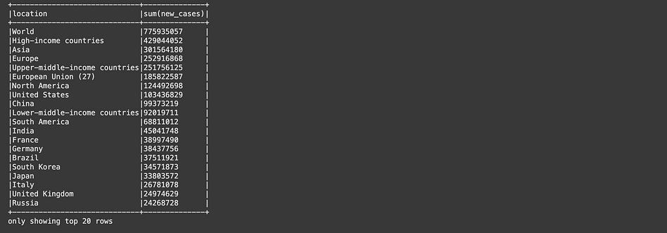
We can also convert this dataframe into an SQL equivilent view, and apply SQL commands to it.
df.createOrReplaceTempView(”covid_data”)

spark.sql(”“”
    SELECT
        location,
        SUM(new_cases) AS total_new_cases
    FROM covid_data
    GROUP BY location
    ORDER BY total_new_cases DESC
“”“).show(truncate=False)
Feel free to check out my article on SQL, if you want to learn more.
Conclusion
Spark has a ton of tooling, and I can’t go in depth into all of it. The main job of this article was to serve as an introduction to Spark, its core paradigms, and what it’s good for. Using these core principles, and a bit of application specific research you can use Spark to do a wide range of large scale data processing operations:
Real time analytics over extremely large datasets
Distributed machine learning and model training
Large-scale data cleaning, feature engineering, and preprocessing
Large-scale ETL pipelines
And so much more. In my mind, Spark doesn’t do much on it’s own. Rather, it’s a quick way to turn your algorithm or technology into a massively parallelized system. Thus, it’s an incredibly usefull tool for developers working with large amounts of data.