
Structured Query Language — Intuitively and Exhaustively Explained
Speaking with Data


In this article we’ll discuss “Structured Query Language” (SQL), the most common language for describing how data is organized, searched, and manipulated. From multi billion dollar companies to mini databases running on smartphones, where there’s data there’s SQL.
SQL is easy to learn and hard to master, which is why this article is so absurdly long. It’s relatively straightforward, but there are a huge number of tricks that can be stitched together to create very complex functionality. We’ll be starting off with the basics, and then we’ll get into queries that would make a senior FAANG developer's head spin. More importantly, though, we’ll show how high-quality SQL queries can do a ton of heavy lifting in building complex applications.
Whether you’re an SQL pro or a complete beginner, you’ll walk away with a much stronger understanding of SQL by reading this article.
-- An example of one of the crazy SQL queries we'll be
-- discussing, line by line, by the end of the article

WITH base AS (
    SELECT *
    FROM trades
    WHERE symbol = 'AAPL'
),

windowed AS (
    SELECT
        id,
        trade_time,
        price,
        volume,
        LAG(price) OVER (ORDER BY trade_time) AS prev_price,
        LEAD(price) OVER (ORDER BY trade_time) AS next_price,
        ROUND(AVG(price) OVER (ORDER BY trade_time ROWS BETWEEN 4 PRECEDING AND CURRENT ROW), 2) AS price_avg_5,
        ROUND(100.0 * (price - LAG(price) OVER (ORDER BY trade_time)) / LAG(price) OVER (ORDER BY trade_time), 2) AS return_pct,
        CASE
            WHEN price > LAG(price) OVER (ORDER BY trade_time) THEN '↑ UP'
            WHEN price < LAG(price) OVER (ORDER BY trade_time) THEN '↓ DOWN'
            ELSE '→ FLAT'
        END AS trend,
        CASE
            WHEN volume > AVG(volume) OVER (ORDER BY trade_time ROWS BETWEEN 4 PRECEDING AND CURRENT ROW) * 1.5 THEN '⚠️ VOLUME SPIKE'
            ELSE ''
        END AS volume_alert,
        CASE
            WHEN price > LAG(price) OVER (ORDER BY trade_time) AND price > LEAD(price) OVER (ORDER BY trade_time) THEN '🔺 LOCAL PEAK'
            WHEN price < LAG(price) OVER (ORDER BY trade_time) AND price < LEAD(price) OVER (ORDER BY trade_time) THEN '🔻 LOCAL DIP'
            ELSE ''
        END AS local_extreme
    FROM base
),

active_window AS (
    SELECT trade_time
    FROM windowed
    GROUP BY strftime('%H:%M', trade_time)
    ORDER BY SUM(volume) DESC
    LIMIT 15
)

SELECT w.trade_time, w.price, w.volume,
       w.trend, w.return_pct || '%' AS return,
       w.price_avg_5 AS "5ma",
       w.volume_alert, w.local_extreme
FROM windowed w
WHERE strftime('%H:%M', w.trade_time) IN (SELECT strftime('%H:%M', trade_time) FROM active_window)
ORDER BY w.trade_time;
Who is this useful for? Anyone who’s passionate about constructing complex queries on enterprise-scale data, or is passionate about making a lot of money.
How advanced is this post? This post is designed to be both beginner accessible in earlier sections, and challenging to senior developers in later sections
Pre-requisites: None
What is SQL
This is an easy question to answer briefly, but it can get pretty complicated if you peek beneath the rug. At the highest level, SQL stands for “structured query language”, and is a language used to communicate with “relational databases”.
A “relational database” consists of pre-defined tables. how many tables there are, and what data is in those tables, is defined by the “schema” of the database. The schema is simply a plan for how the database is structured.

These types of databases are “relational” because the tables usually reference each other in some way. A customer ID, might be referenced in a transaction for a purchasing database in a supermarket, for instance.
“Structured Query Language” is a language for communicating with this type of data. Creating new tables, new “records” (rows) in the tables, doing some analytical work with the data, etc.
That’s where a lot of descriptions end, but in the spirit of “Exhaustively Explained”, let’s peek beneath the rug to talk about what SQL really is.
What SQL really is
SQL is a “declarative language”, meaning, instead of telling a computer how to manipulate data, you’re telling a computer what you want. Take the following snippet of SQL code, for instance:
SELECT name FROM customers WHERE age > 30;Here, we’re saying we want the name for every customer in a table called customers where that customer has an age greater than 30. We “declare” that we want this information, then this declaration is passed to an “database engine” that will accept our SQL and get us what we want.
There are many database engines (like PostgreSQL, SQLite, MySQL, or SQL Server), and their job is to accept SQL commands and execute them as efficiently as possible. Generally speaking these engines have different costs and benefits, and are designed to meet different use cases:
SQLite is a lightweight, embedded SQL engine with minimal setup and a relaxed interpretation of types.
PostgreSQL is standards-compliant and highly extensible
MySQL is widely used in web applications and emphasizes speed, sometimes at the expense of strict SQL compliance.
SQL Server by Microsoft uses T-SQL, which is SQL + proprietary extensions.
Each of these SQL engines accepts the same core functionality, but might expand on it in some way. Thus, certain advanced SQL commands, might not be compatible with every database engine.
That said, they all obey the same core rules of SQL, and the vast majority of SQL written for these engines is cross-compatible. So, with some exceptions, SQL is a portable way to communicate with these database engines.
In being a high level declaration, SQL’s grammatical structure is, fittingly, fairly high level. It’s kind of a weird, super rigid version of English. SQL queries are largely made up of:
Keywords: special words in SQL that tell an engine what to do. Some common ones, which we’ll discuss, are
SELECT, FROM, WHERE, INSERT, UPDATE, DELETE, JOIN, ORDER BY, GROUP BY. They can be lowercase or uppercase, but usually they’re written in uppercase.Identifiers: Identifiers are the names of database objects like tables, columns, etc.
Literals: numbers, text, and other hardcoded values
Operators: Special characters or keywords used in comparison and arithmetic operations. For example
!=,<,OR,NOT,*,/,%,IN,LIKE. We’ll cover these later.Clauses: These are the major building block of SQL, and can be stitched together to combine a queries general behavior. They usually start with a keyword, like
SELECT– defines which columns to returnFROM– defines the source tableWHERE– filters rowsGROUP BY– groups rows
etc.
By combining these clauses, you create an SQL query. Here’s an example:
SELECT name, COUNT(*)
FROM users
WHERE active = TRUE
GROUP BY name
HAVING COUNT(*) > 1
ORDER BY name
LIMIT 5;
Functions: These are routines that do some standard operation, like adding things up (
SUM), counting how many rows (records) there are (COUNT), etc.
When you create a “statement” in SQL (a statement being a complete instruction), that gets sent to whatever database engine you’re connected to. The database engine then parses out the text into a known structure (SQL accepts a fairly loose textual structure, so the database engine has to unravel that structure and turn it into something consistent) and checks if your query makes sense (are you talking about a table that actually exists, for instance). It then comes up with a set of operations to get you the result you want. This is a whole can of worms within itself that you don’t have to touch. You just send your SQL to the engine, and it figures out how to optimally execute operations to get you what you want.
To make things easy on ourselves, we’re going to be using SQLite in this tutorial. SQLite is the most widely deployed database engine in the world, largely because it’s small, fast, self-contained, and highly reliable.
When most people think SQL they think of a database, a server and all sorts of complicated online stuff. That’s certainly a common application, but SQLite is designed to be spooled up and run locally, meaning you can create and connect to a database on a single machine. This is handy if you’re developing… Well, pretty much anything. SQLite is deployed on:
- Every Android device
- Every iPhone and iOS device
- Every Mac
- Every Windows10 machine
- Every Firefox, Chrome, and Safari web browser
- Every instance of Skype
- Every instance of iTunes
- Every Dropbox client
- Every TurboTax and QuickBooks
- PHP and Python
- Most television sets and set-top cable boxes
- Most automotive multimedia systems
- Countless millions of other applications…
SQLite is probably one of the top five most deployed software modules of any description- source
Data scientists spend most of their time playing around with database engines like PostgreSQL or MySQL, which are designed to handle massive workloads in large enterprises. That said, the SQL for all these engines is 99% the same, and SQLite has the benefit of being dirt simple to set up, so that’s why we’ll be using it.
If you’ve been reading my articles for a while, you can probably guess where we’ll be running our code :)
Setting up SQLite on Google Colab
Full code can be found here.
For the uninitiated, Google Colab is a place python code can be run. I have an entire article on how Google Colab works, if you’re interested:

Python has a handy little library called sqlite3 which can be used to spool up databases, execute SQL queries, and get back responses using SQLite. We’ll essentially be using sqlite3 as a lightweight wrapper around our SQLite to get our SQL to actually do stuff.
When you call the sqlite3.connect command, a file gets created that represents your database. You then create a cursor that’s used to edit that file.
import sqlite3
connection = sqlite3.connect("tutorial.db")
cursor = connection.cursor()
You run SQL by telling the cursor you want to edit the file based on an SQL query. For example:
cursor.execute("""

CREATE TABLE movie(title, year, score)

""")
(You don’t have to understand the code in this section, we’ll be covering these topics later. The purpose of this section is to introduce the workflow we’ll be using from a high level).
Sometimes you need to call the cursor.commit function to actually do the changes, like when you’re adding stuff to a table.
cursor.execute("""

INSERT INTO movie VALUES
    ('Monty Python and the Holy Grail', 1975, 8.2),
    ('And Now for Something Completely Different', 1971, 7.5)

""")
connection.commit()
When you want to get data out of your database, it gets returned as python objects, which is cool but it’s not super easy to interpret.
res = cursor.execute("""

SELECT score FROM movie

""")
res.fetchall()
As a result, I made two helper functions: one that can render a table in the database by name,
import sqlite3
from IPython.display import Markdown, display

def display_table(cursor, table_name):

    # Getting all the content from a table
    cursor.execute(f"""

    SELECT * FROM {table_name}

    """)
    rows = cursor.fetchall()
    columns = [description[0] for description in cursor.description]

    # Building a markdown table
    md = "| " + " | ".join(columns) + " |\n"
    md += "| " + " | ".join(["---"] * len(columns)) + " |\n"
    for row in rows:
        md += "| " + " | ".join(str(cell) for cell in row) + " |\n"

    # Displaying in Markdown format
    display(Markdown(md))


display_table(cursor, "People")
and one that renders the result of a query.
from tabulate import tabulate

def display_results(cursor, results):

    # Get column names from cursor.description
    columns = [desc[0] for desc in cursor.description]

    # Render Markdown table
    display(Markdown((tabulate(results, headers=columns, tablefmt="github"))))

display_results(cursor, results)
I don’t want to get into exactly how these helper functions work, it’s not really relevant to the core idea of the article. Still, though, I wanted to introduce them early because we’ll be relying on them throughout the article.
If all that went over your head, don’t sweat it. Let’s get into the basics of SQL.
Creating a Simple Database
First off, we need to create an SQLite database.
import sqlite3
connection = sqlite3.connect("example_database_1.db")
cursor = connection.cursor()
the sqlite3.connect function either creates a new database file, or accesses an existing one. Here, we’ll be creating a new file. If you want to re-run some code from scratch, you can always just delete the database file.
In that database let’s create a table called People
cursor.execute("""

CREATE TABLE People(first_name, last_name, age, favorite_color)

""")
By convention, table names are plural because they contain multiple records. So, the “People” table contains many individual people.
Here, a person is defined as a first name, last name, age, and favorite color. We can populate our table with a few records in the following way:
cursor.execute("""

INSERT INTO People
VALUES
    ('Tom', 'Sawyer', 19, 'White'),
    ('Mel', 'Gibson', 69, 'Green'),
    ('Daniel', 'Warfiled', 27, 'Yellow')

""")
connection.commit()
The INSERT INTO keyword allows you to specify a table you want to insert values into, then you can specify the VALUES of each record you want to add.
We can get our content from our table with the following:
cursor.execute(f"""

SELECT * FROM People

""")
results = cursor.fetchall()
display_results(cursor, results)
Here, SELECT * FROM People means we want to get all of the columns, denoted with * , from the People table in the database. cursor.fetchall gets our results into python and display_results is our helper function that renders a table.
We don’t have to get all columns, we can also specify columns by name.
cursor.execute(f"""

SELECT first_name, favorite_color FROM People

""")
results = cursor.fetchall()

display_results(cursor, results)
Playing around a bit more, we can add a person (AKA a row, AKA a record) to our table with a NULL value. NULL means that there’s no value for a particular column within a record.
cursor.execute("""

INSERT INTO People
VALUES
    ('Tom', 'Bombadil', NULL, 'Yellow')

""")
connection.commit()
Tom Bombadil is an ageless character from the Lord Of The Rings. Depending on the context, it might make sense to define his age as NULL , in other contexts it might make sense to define his age as a really big number, or -1 . The exact specifics of how you choose to represent these types of subtleties has a lot to do with the application you’re building the database for.
We can render out our table with our helper function:
display_table(cursor, "People")
Here, our python library sqlite3 recognizes NULL in SQL and turns it into the equivalent python value None.
If you’re new to SQL I highly recommend spooling up a colab notebook and playing around with it; SQL is much easier to learn as an active participant. Let’s explore how we can search through our database.
Basic Search
Let’s create a new database with some more fields.
# creating the database
import sqlite3
connection = sqlite3.connect("example_database_2.db")
cursor = connection.cursor()

# creating a table
cursor.execute("""

CREATE TABLE People(
    id INTEGER PRIMARY KEY,
    first_name TEXT,
    last_name TEXT,
    age INTEGER,
    favorite_color TEXT
)

""")

# adding data to the table
cursor.execute("""

INSERT INTO People
VALUES
    (NULL, 'Tom', 'Sawyer', 19, 'White'),
    (NULL, 'Mel', 'Gibson', 69, 'Green'),
    (NULL, 'Daniel', 'Warfiled', 27, 'Yellow')

""")
connection.commit()

# Rendering the table
display_table(cursor, "People")
I snuck a new idea into this table, called a PRIMARY KEY . Primary keys are a super important concept in relational databases, and serves as a unique identifier for each record in a table. In SQLite, if you specify that a column has type INTEGER and is a PRIMARY KEY , SQLite will auto increment that value when you add records, which is handy.
You might notice that I specified some other data types, like TEXT and INTEGER. In SQLite this is pretty much just for aesthetics, SQLite doesn’t have any strict type enforcement, so we can do weird stuff like this if we really want to:
# adding a weird row
cursor.execute("""

INSERT INTO People
VALUES
    (NULL, 3, 3, 'hello', 3)

""")
connection.commit()

# rendering
display_table(cursor, "People")
To me, this kind of makes sense. SQLite is designed for local and embedded systems, and the ease of use of a dynamically typed system is probably tremendously helpful when building applications around SQLite. If you’re facebook, though, and you have a massive database consisting of many, many tables each of which has many, many columns and records, the flexibility of dynamic typing would probably be problematic. For enterprise cloud-centric SQL Engines, like PostgreSQL, stricter type enforcement rules are both possible and considered best practice.
Now that we have an unique id associated with each record, we can look up a particular record by it’s id.
cursor.execute("""

SELECT * FROM People WHERE id = 3

""")
results = cursor.fetchall()
display_results(cursor, results)
Here, I’m getting all columns ( SELECT * FROM People ) for the records WHERE id = 3 . I mentioned earlier that SQL accepts a pretty broad spread of formatting options. You could also write the same statement like this:
SELECT *
FROM People WHERE id = 3
or like this
SELECT
  *
FROM
  People WHERE id = 3
or even like this, though I don’t know why you’d want to.
SELECT
*
FROM
People
WHERE
id
=
3
The parser in whatever SQL engine you’re using should be able to deal with it, as long as you’re using newlines and spaces in a way that’s even remotely reasonable.
We don’t have to filter by ID. We could also filter by age, for instance.
"""Getting the first and last name of all people under the age of 30
"""

cursor.execute("""

SELECT first_name, last_name FROM People WHERE age < 30

""")
results = cursor.fetchall()
display_results(cursor, results)
Recall that we created that weird row earlier. It has the text “hello” where the age should be, which can result in some weird output.
"""Getting people over the age of 20
"""

cursor.execute("""

SELECT * FROM People WHERE age > 20

""")
results = cursor.fetchall()
display_results(cursor, results)
So, we can create a table in a database, add data to it, and do some simple searches. That’s actually enough for some applications, but there’s one more essential database operation we haven’t covered.
Deletion
Just to keep things clean, let’s spool up a new database.
import sqlite3
connection = sqlite3.connect("example_database_3.db")
cursor = connection.cursor()

cursor.execute("""

CREATE TABLE People(
    id INTEGER PRIMARY KEY,
    first_name TEXT,
    last_name TEXT,
    age INTEGER,
    favorite_color TEXT
)

""")

cursor.execute("""

INSERT INTO People
VALUES
    (NULL, 'Tom', 'Sawyer', 19, 'White'),
    (NULL, 'Mel', 'Gibson', 69, 'Green'),
    (NULL, 'Daniel', 'Warfiled', 27, 'Yellow')

""")
connection.commit()

display_table(cursor, "People")
Instead of SELECTing data, we can DELETE data
cursor.execute("""

DELETE FROM People WHERE age < 30

""")
connection.commit()

display_table(cursor, "People")
We can also delete tables by name with the DROP keyword
# Drop the table
cursor.execute("""

DROP TABLE IF EXISTS People

""")
connection.commit()
If we try to render out the People table, we’ll get an error due to the table no longer existing.
display_table(cursor, "People")
And that covers, in my opinion, the bare necessities of SQL. If you know how to create tables, add data to those tables, search through data, and delete stuff, you can do a lot. As you can probably tell from the length of this post, though, we’re just scratching the surface.
Defining Relationships with Primary and Foreign Keys, and Introducing Entity Relationships
Recall that SQL is designed to interface with “relational” databases. “Primary” and “foreign” keys are the things that make these databases “relational”.
A “Primary Key” is a unique identifier that gets assigned to each record in a table. Most commonly, this takes the form of an index or a unique identifier (UID). that gets assigned to each record automatically upon creation.
==============
Comments Table
==============
UID              Comment
"aflioi128-09" , "Hello"
"9khida87kh1n" , "My name is Daniel"
"-80yadjgkawu" , "These are entries in a DataBase"
The most common scheme for unique identification is the “Universal Unique Identifier” (UUID), which is a 128 bit randomly generated string. Because it’s sufficiently long, anyone that generates a UUID is likely generating the only one, ever, in existence.
# an example of a UUID
"f81d4fae-7dec-11d0-a765-00a0c91e6bf6"
In formal relational database terms, there’s also an idea called a “super key”. Primary keys must be unique within a table, but super keys allow you to define two or more columns which, together, are unique.
==============
Comments Table
==============
User,      UNIX_Time   Comment
"Daniel",  1744113162, "Hey"
"Bob",     1744113162, "Hello"
"Daniel",  1744113162, "Oh, wow, we sent that at the same time!"
Here, the “User” and “Unix_Time”, together, might make up the “super key” (also known as a composite key).
Super keys are a usefull concept to know; the idea that two columns together might be unique is powerfull. That said, practically, ommitting a unique identifier that easily isolates individual records often results in more trouble than it’s worth. Therefore, it’s customary to assign a unique ID to each record, either in terms of a UUID
==============
Comments Table
==============
UUID,                   User,      UNIX_Time   Comment
"f81d4fae....f81d4fae", "Daniel",  1744113162, "Hey"
"ihjl90da....awilh08k", "Bob",     1744113162, "Hello"
"89712hbn....080hoihb", "Daniel",  1744113162, "Oh, wow, we sent that at the same time!"
or perhaps in terms of some incrementing index, as we defined previously.
==============
Comments Table
==============
index,  User,      UNIX_Time   Comment
0,     "Daniel",  1744113162, "Hey"
1,     "Bob",     1744113162, "Hello"
2,     "Daniel",  1744113162, "Oh, wow, we sent that at the same time!"
The existence of primary keys allows for the existence of “foreign keys”. Foreign keys are when a table references some other table by it’s primary key.
For instance, imagine if we had two tables. One for users, and one for chat.
==============
Users
==============
Index,  First_Name, Last_Name
0,     "Daniel",  "Warfield"
1,     "Saul",    "Goodman"

==============
CommentsTable
==============
Index,  User,     UNIX_Time   Comment
0,      0,        1744113162, "Hey"
1,      1,        1744113162, "Hello"
2,      1,        1744113162, "Oh, wow, we sent that at the same time!"
Here the Index in the Users table is the primary key, and the User in the CommentsTable is the foreign key, which references the Index in the Users table. Thus, we can look up things like the users first name for a particular comment by using the foreign key in the CommentsTable to look up information in the Users table.
The separation of data into separate tables is important because it minimizes duplicate information, and generally makes databases more robust. The general idea of making databases more robust by separating out information is called “Normalization”, and can be done to a variety of degrees called “Forms”.
Unnormalized Form might look like this, a table with everything in it:
StudentCourses
+----+--------+---------------------------+-----------------------------+------------------+
| ID | Name   | Courses                   | Instructors                 | Departments      |
+----+--------+---------------------------+-----------------------------+------------------+
| 1  | Alice  | Math, Physics             | Dr. Smith, Dr. Lee          | Math, Physics    |
| 2  | Bob    | Math, Chemistry, Biology  | Dr. Smith, Dr. Chen, Dr. Ray| Math, Chemistry, Biology |
+----+--------+---------------------------+-----------------------------+------------------+
First Normal Form removes groups from columns, making each row atomic:
StudentCourses_1NF
+----+--------+----------+-------------+-------------+
| ID | Name   | Course   | Instructor  | Department  |
+----+--------+----------+-------------+-------------+
| 1  | Alice  | Math     | Dr. Smith   | Math        |
| 1  | Alice  | Physics  | Dr. Lee     | Physics     |
| 2  | Bob    | Math     | Dr. Smith   | Math        |
| 2  | Bob    | Chemistry| Dr. Chen    | Chemistry   |
| 2  | Bob    | Biology  | Dr. Ray     | Biology     |
+----+--------+----------+-------------+-------------+
Second Normal Form states that tables should be separated such that only one key thing should be represented in each table. Here, we have courses and students in the same table. This can be divided into two tables.
Students
+----+--------+
| ID | Name   |
+----+--------+
| 1  | Alice  |
| 2  | Bob    |
+----+--------+

Enrollments
+----+----------+-------------+-------------+
| ID | Course   | Instructor  | Department  |
+----+----------+-------------+-------------+
| 1  | Math     | Dr. Smith   | Math        |
| 1  | Physics  | Dr. Lee     | Physics     |
| 2  | Math     | Dr. Smith   | Math        |
| 2  | Chemistry| Dr. Chen    | Chemistry   |
| 2  | Biology  | Dr. Ray     | Biology     |
+----+----------+-------------+-------------+
Here, Students.ID is the primary key for each student, and Enrollments.ID is a foreign key which references Students.ID . In this particular example, (ID, Course) makes up a composite key which uniquely represents each record in the Enrollments Table.
In second normal form, the course information like Instructor and Department was included in the Enrollments .In third normal form, this would be separated.
Students
+----+--------+
| ID | Name   |
+----+--------+
| 1  | Alice  |
| 2  | Bob    |
+----+--------+

Courses
+----------+-------------+-------------+
| Course   | Instructor  | Department  |
+----------+-------------+-------------+
| Math     | Dr. Smith   | Math        |
| Physics  | Dr. Lee     | Physics     |
| Chemistry| Dr. Chen    | Chemistry   |
| Biology  | Dr. Ray     | Biology     |
+----------+-------------+-------------+

Enrollments
+----+----------+
| ID | Course   |
+----+----------+
| 1  | Math     |
| 1  | Physics  |
| 2  | Math     |
| 2  | Chemistry|
| 2  | Biology  |
+----+----------+
I’ll be honest, I find the specifics of the various normal forms to be excessively pedantic. If you’re working on massive databases with huge numbers of tables, then formal rigidity about these definitions is critical. If you’re a normal developer, though, a general understanding of these ideas is likely sufficient.
Really, the big takeaway is that the usage of primary keys and foreign keys allow one to split data across multiple tables, which is how “Relational Databases” got their name.
We can define a database with a few tables, and define their relationships with the following:
import sqlite3

connection = sqlite3.connect("schema_tutorial.db")
cursor = connection.cursor()

cursor.executescript("""
DROP TABLE IF EXISTS comments;
DROP TABLE IF EXISTS posts;
DROP TABLE IF EXISTS users;

CREATE TABLE users (
    id INTEGER PRIMARY KEY,
    name TEXT NOT NULL,
    email TEXT UNIQUE NOT NULL
);

CREATE TABLE posts (
    id INTEGER PRIMARY KEY,
    title TEXT NOT NULL,
    content TEXT,
    user_id INTEGER,
    FOREIGN KEY (user_id) REFERENCES users(id)
);

CREATE TABLE comments (
    id INTEGER PRIMARY KEY,
    text TEXT,
    post_id INTEGER,
    user_id INTEGER,
    FOREIGN KEY (post_id) REFERENCES posts(id),
    FOREIGN KEY (user_id) REFERENCES users(id)
);
""")

connection.commit()
If you try to create a table that already exists then you’ll be met with an error, so I’m dropping all the tables if they already exist. This is handy if I want to re-run the same code block numerous times.
DROP TABLE IF EXISTS comments;
DROP TABLE IF EXISTS posts;
DROP TABLE IF EXISTS users;
Then, I’m creating a table for users with an auto-incrementing id, like we did in a previous example
CREATE TABLE users (
    id INTEGER PRIMARY KEY,
    name TEXT NOT NULL,
    email TEXT UNIQUE NOT NULL
);
I’m also specifying some constraints for this table. The name can NOT be NULL , and the email has to be UNIQUE . Unlike datatypes like INTEGER and TEXT , which SQLite does not strictly enforce, SQLite does strictly enforce NOT NULL and UNIQUE , so if we try to create two users with the same email we’ll get an error.
I’m also creating a table called posts . This might be for a social media app like Twitter, for instance.
CREATE TABLE posts (
    id INTEGER PRIMARY KEY,
    title TEXT NOT NULL,
    content TEXT,
    user_id INTEGER,
    FOREIGN KEY (user_id) REFERENCES users(id)
);
Here, I’m saying each post has an id , title , content , and user_id . I’m also specifying explicitly that the user_id is a FOREIGN KEY that references the id column in the users table.
By specifying explicitly that user_id is a foreign key, We can enable rules, like SQLite checking that a corresponding users.id exists. If we enabled that rule, and the corresponding users.id doesn’t exist, an error would be thrown. There’s also advanced stuff you can do here, like enabling delete cascades, which will automatically delete posts that point to a user that’s been deleted.
CREATE TABLE posts (
  ...
  FOREIGN KEY (user_id) REFERENCES users(id) ON DELETE CASCADE
);
Here, the user_id REFERENCES the id in users . ON DELETE of a user in users , the DELETE CASCADEs to all the posts that point to that user by users.id .
Let’s make one more table, one for comments. This has two foreign keys, one that points to the user making the comment, and one for the post for that comment.
CREATE TABLE comments (
    id INTEGER PRIMARY KEY,
    text TEXT,
    post_id INTEGER,
    user_id INTEGER,
    FOREIGN KEY (post_id) REFERENCES posts(id),
    FOREIGN KEY (user_id) REFERENCES users(id)
);
You might notice the inclusion of ; in this example, which we didn’t previously use. sqlite3 , our python library we’re using to run SQLite, has two major functions for running SQL:
cursor.executeruns a single SQL Statementcursor.executescriptruns an SQL Script
SQL Scripts can have numerous statemtnts. We conclude a statement with ; .
Now that we have three tables with primary and foreign keys specified, we can draw something called an “Entity Relationship Diagram”. This is a diagram that shows what tables exist, and how they relate with one another. We’ll use a library called sqlalchemy to load up our table definitions from our database file, and eralchemy to render an entity relationship diagram based on those definitions
from sqlalchemy import create_engine, MetaData
from eralchemy import render_er

# loading table definitions
engine = create_engine('sqlite:///schema_tutorial.db')
metadata = MetaData()
metadata.reflect(bind=engine)

# Render ER diagram
render_er(metadata, 'erd_from_sqlite.png')
Notice that there are dotted lines between the primary and foreign keys within the various tables. Here {0,1} and 0..N represent “cardinality” which describes how many rows in one table can be associated with rows in another table.
For Users and Posts, a single user can write many posts, or they might not write any at all. Each post is linked to one user at most, but it could also be unlinked (if
user_idis NULL).For Posts and Comments, apost can have many comments, or none. Each comment is linked to just one post, or possibly none if
post_idis NULL.For Users and Comments, a user can write lots of comments, or none. Each comment can be connected to one user, or possibly not connected at all.
In different SQL Engines, these entity relationship diagrams can be adjusted more or less rigidly, with various forms of cardinality being supported.
Let’s use this idea of relationships to do stuff.
Joins
Let’s whip up a new example
import sqlite3
connection = sqlite3.connect("example_database_5.db")
cursor = connection.cursor()

cursor.executescript("""

CREATE TABLE Users(
    id INTEGER PRIMARY KEY,
    username TEXT
);

CREATE TABLE Comments(
    id INTEGER PRIMARY KEY,
    comment TEXT,
    user_id INTEGER,
    FOREIGN KEY (user_id) REFERENCES Users(id)
);

INSERT INTO Users (id, username) VALUES
    (NULL, 'alice'),
    (NULL, 'bob'),
    (NULL, 'charlie'),
    (NULL, 'quiet guy');

INSERT INTO Comments (id, comment, user_id) VALUES
    (NULL, 'Hello world!', 1),
    (NULL, 'Nice to meet you.', 1),
    (NULL, 'This is a comment.', 2),
    (NULL, 'Another one here.', 3),
    (NULL, 'Final test comment.', 3),
    (NULL, 'Ghost Comment', NULL);

""")
connection.commit()
Here we’re creating two tables, one for Users and one for Comments. We’re also populating those tables with some information. Let’s take a look at those tables and see what we get.
print('Users:')
display_table(cursor, "Users")
print('\nComments:')
display_table(cursor, "Comments")
“JOIN” is a fundamental idea in SQL that allows one to join tables based on the relationship of primary and foreign keys. Because Comments references Users by user_id , we can do a join with the following:
cursor.execute("""

SELECT
    Users.username,
    Comments.comment
FROM Comments
JOIN Users ON Comments.user_id = Users.id

""")

results = cursor.fetchall()
display_results(cursor, results)
You can think of this as constructing a new table, where we JOIN the Comments table with the Users table where Comments.user_id is equal to Users.id . Then, we display the username from Users and the comment from Comments for each of those rows with the SELECT statement.
JOIN ignores values that don’t have an association. In our database, the user quiet guy doesn’t have any comments, and the comment ghost comment doesn’t have a corresponding user, so they don’t show up in the JOIN .
If we wanted to show comments that don’t have any associated users, we could use LEFT JOIN , which preserves every row that’s being joined onto.
Here, we’re joining Users onto Comments , because Comments is on the left of the JOIN statement.
FROM Comments JOIN Users ON Comments.user_id = Users.idSo, if we used LEFT JOIN , we would preserve all comments (even those with no user), and then join our users onto it.
cursor.execute("""

SELECT
    Users.username,
    Comments.comment
FROM Comments
LEFT JOIN Users ON Users.id = Comments.user_id

""")

results = cursor.fetchall()
display_results(cursor, results)
This is a little confusing, because the comments are on the right, but that’s dictated by the order of the SELECT statement.
In some SQL Engines, if we wanted to show the all usernames that don’t have any comments attached, we might turn our LEFT JOIN into a RIGHT JOIN , like so:
FROM Comments RIGHT JOIN Users ON Users.id = Comments.user_idThis would join Users onto Comments while preserving all Users , rather than all Comments .
SQLite doesn’t have a RIGHT JOIN , but we can emulate this effect by simply swapping the order of our tables in the LEFT JOIN statement.
cursor.execute("""

SELECT
    Users.username,
    Comments.comment
FROM Users
LEFT JOIN Comments ON Users.id = Comments.user_id

""")

results = cursor.fetchall()
display_results(cursor, results)
Here, we’re LEFT JOINing Users into Comments , instead of the other way around, so quiet guy shows up, instead of Ghost Comment .
In a lot of SQL Engines there’s also the idea of a “FULL OUTER JOIN”, which preserves NULL values from both sides of the JOIN . SQLite (or, at least the version I’m using) doesn’t support full outer join, but we can emulate it using UNION and WHERE .
cursor.execute("""

SELECT
    Comments.comment,
    Users.username
FROM Comments
LEFT JOIN Users ON Comments.user_id = Users.id

UNION

SELECT
    Comments.comment,
    Users.username
FROM Users
LEFT JOIN Comments ON Users.id = Comments.user_id
WHERE Comments.user_id IS NULL

""")

results = cursor.fetchall()
display_results(cursor, results)
In most SQL Engines, like PostgreSQL or SQL Server, you would just do
SELECT
    Comments.comment,
    Users.username
FROM Comments
FULL OUTER JOIN Users ON Comments.user_id = Users.id;
This uses two new keywords, UNION and WHERE . UNION is straight forward, you just combine two tables together, we’ll cover it more later. WHERE is a bit more complicated, we’ll discuss it in the next section.
Filtration with Where, and Limiting
The WHERE keyword allows us to filter data in SQL. We can use the database we defined in the last section to search for a particular user by their id
print('Original Users Table:')
display_table(cursor, "Users")

#filtering by user id using WHERE

cursor.execute("""

SELECT * FROM Users
WHERE id = 2

""")

results = cursor.fetchall()
print('\nFiltered Users Table:')
display_results(cursor, results)
It’s pretty straight forward, we’re getting all the columns for the Users table (SELECT * FROM Users), but only for records WHERE id = 2.
Let’s spool up more data so we can play around with WHERE statements that are a bit less trivial.
import sqlite3
import random
import string

# Connect to an in-memory SQLite database
connection = sqlite3.connect("example_database_7.db")
cursor = connection.cursor()

# Create the employees table
cursor.execute("""
CREATE TABLE employees (
    id INTEGER PRIMARY KEY,
    name TEXT,
    department TEXT,
    age INTEGER,
    salary REAL,
    full_time BOOLEAN
)
""")

# Generate random data
departments = ['Engineering', 'Sales', 'HR', 'Marketing', 'Support']
def random_name():
    return ''.join(random.choices(string.ascii_uppercase, k=1)) + ''.join(random.choices(string.ascii_lowercase, k=6))

data = [
    (
        i,
        random_name(),
        random.choice(departments),
        random.randint(20, 65),
        round(random.uniform(40000, 120000), 2),
        random.choice([0, 1])
    )
    for i in range(1, 50)
]

# Insert data into the table
cursor.executemany("INSERT INTO employees VALUES (?, ?, ?, ?, ?, ?)", data)
connection.commit()
Here I’m doing a bunch of python and sqlite3 specific stuff, so I don’t want to get too into the weeds, but I’m basically just generating a big random table of employees.
print('Original Users Table:')
display_table(cursor, "employees")
This table is 49 rows long, and has information about employees, their department, age, salary, and weather or not they’re full time.
We can use the WHERE keyword to filter by engineers under the age of 30, for instance.
print("\nEmployees in Engineering under age 30:")
results = cursor.execute("SELECT * FROM employees WHERE department = 'Engineering' AND age < 30")
display_results(cursor, results)
Here we’re using the AND keyword to search for records where department = ‘Engineering’ AND age < 30
We can also search for people who earn over 100,000 . There might be a lot of them, so we can LIMIT our results to 5 records or less.
print("\nPart-time employees in Sales:")
results = cursor.execute("SELECT * FROM employees WHERE department = 'Sales' AND full_time = 0 LIMIT 5")
display_results(cursor, results)
We can search for 5 part time employees in sales
print("\nPart-time employees in Sales:")
results = cursor.execute("SELECT * FROM employees WHERE department = 'Sales' AND full_time = 0 LIMIT 5")
display_results(cursor, results)
etc. You get the idea.
Different datatypes have different functionality for comparison. You can search a column of strings based on regular expressions, you can filter records based on time; there’s a lot, and other SQL Engines have even more.
"""Making a database with a variety of datatypes
"""

# Connect to an in-memory SQLite database
connection = sqlite3.connect("example_database_8.db")
cursor = connection.cursor()

# Create a table showing off common SQL data types
cursor.execute("""
CREATE TABLE datatypes_demo (
    id INTEGER PRIMARY KEY,
    age INTEGER,                  -- Whole numbers
    height REAL,                  -- Decimal numbers
    name TEXT,                    -- Strings
    profile_picture BLOB,        -- Binary large object
    is_active NUMERIC,           -- Often used for BOOLEAN (0/1)
    created_at TEXT              -- ISO format date/time as TEXT
);
""")

# Insert one row using all types
cursor.execute("""
INSERT INTO datatypes_demo (age, height, name, profile_picture, is_active, created_at)
VALUES (
    30,                          -- INTEGER
    5.9,                         -- REAL
    'Alice Smith',              -- TEXT
    X'89504E470D0A1A0A',         -- BLOB (mock PNG header)
    1,                           -- NUMERIC as BOOLEAN (1 = True)
    '2025-04-05T15:30:00'        -- TEXT for date/time
);
""")

print('Datatype Table:')
display_table(cursor, "datatypes_demo")
String comparison has some of the most robust and complex functionality when it comes to comparison. I won’t cover all the operations you can do with strings, but we can go over a few examples. We can filter a based on string equivalence
WHERE name = 'alice'filter by values that are not equal
WHERE name != 'Bob'filter by substring
WHERE name LIKE 'A%'     -- starts with A
WHERE name LIKE '%ice'   -- ends with 'ice'
WHERE name LIKE '%li%'   -- contains 'li'
filter by strings that don’t contain a substring
WHERE name NOT LIKE '%admin%'search using regular expressions
WHERE name REGEXP '^[A-Z][a-z]+$'search if a string is in a set of strings
WHERE status IN ('active', 'pending', 'suspended')And more. Like many coding languages, knowing is 90% of the battle, and being able to Google/ChatGPT is the other 10%.
Distinct Selection
Sometimes you might have a table that has multiple instances of a value in a column, and you want to only select unique examples of that thing. Let’s say we had a table of student’s grades, and we only wanted to see which unique grades existed across all students.
import sqlite3

connection = sqlite3.connect("example_database_9")
cursor = connection.cursor()

# Create table and insert values — all SQL
cursor.executescript("""
-- Create a table of students with possible duplicate grades
CREATE TABLE students (
    id INTEGER PRIMARY KEY,
    name TEXT,
    grade TEXT
);

-- Insert values (some duplicate grades)
INSERT INTO students (name, grade) VALUES
  ('Alice', 'A'),
  ('Alice', 'A'),
  ('Alice', 'D'),
  ('Bob', 'B'),
  ('Charlie', 'A'),
  ('Diana', 'C'),
  ('Ethan', 'B');
""")

print("All grades (including duplicates):")
results = cursor.execute("SELECT grade FROM students")
display_results(cursor, results)
We can modify our SELECT statement by including the DISTINCT keyword, to only SELECT DISTINCT grades.
print("\nDistinct grades (duplicate grades removed):")
results = cursor.execute("SELECT DISTINCT grade FROM students")
display_results(cursor, results)
If we wanted to find every distinct grade from every student, we might use DISTINCT name, grade, which both selects the name and grade columns and returns DISTINCT combinations of the two.
print("\nDistinct combinations of name and grade:")
results = cursor.execute("SELECT DISTINCT name, grade FROM students")
display_results(cursor, results)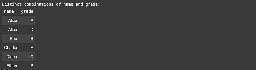
Grouping and Functions
A common application of SQL is to group things, then compute aggregates from those groups. For instance, in the following table:
import sqlite3

connection = sqlite3.connect("example_database_10")
cursor = connection.cursor()

cursor.executescript("""
-- Create a table of employees
CREATE TABLE employees (
    id INTEGER PRIMARY KEY,
    name TEXT,
    department TEXT,
    role TEXT,
    location TEXT,
    salary REAL,
    hire_date TEXT  -- Stored as 'YYYY-MM-DD'
);

-- Insert sample data
INSERT INTO employees (name, department, role, location, salary, hire_date) VALUES
  ('Alice',   'Engineering', 'Developer', 'NY', 95000, '2020-06-15'),
  ('Bob',     'Engineering', 'Developer', 'NY', 92000, '2019-03-20'),
  ('Charlie', 'Engineering', 'Manager',   'SF', 120000, '2018-09-01'),
  ('Diana',   'Marketing',   'Analyst',   'NY', 70000, '2021-02-10'),
  ('Ethan',   'Marketing',   'Manager',   'SF', 105000, '2017-11-05'),
  ('Fay',     'Sales',       'Rep',       'TX', 65000, '2021-07-22'),
  ('Grace',   'Sales',       'Rep',       'TX', 64000, '2022-01-15'),
  ('Henry',   'Sales',       'Manager',   'NY', 99000, '2016-04-30');
""")

display_table(cursor, 'employees')
If we wanted to print the average salary by each department, we could use the following expression:
print('Average salary by department')
results = cursor.execute("""
SELECT department, AVG(salary) AS avg_salary
FROM employees
GROUP BY department;
""")
display_results(cursor, results)
In this expression, we’re GROUPing BY department in the employees table, and then displaying the department and AVG (average) of the salary of each department (which we GROUP BYd with), and displaying that average salary as avg_salary.
When a GROUP BY is not specified, functions like AVG (average), SUM , and COUNT work globally across the entire table. When a GROUP BY is specified, these functions operate over each individual group.
We can filter this data using the average salary of each group, using the following:
print('Average salary by department')
results = cursor.execute("""
SELECT department, AVG(salary)
FROM Employees
GROUP BY department
HAVING AVG(salary) > 80000;
""")
display_results(cursor, results)
We can use the COUNT to count how many employees there are in each role:
print('Number of employees per roll')
results = cursor.execute("""
SELECT role, COUNT(*) AS num_employees
FROM employees
GROUP BY role;
""")
display_results(cursor, results)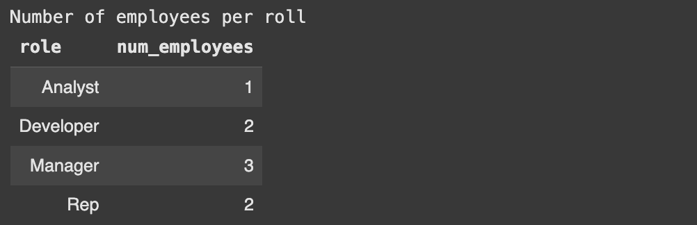
We can sum up the salary per location
print('Total salary per location')
results = cursor.execute("""
SELECT location, SUM(salary) AS total_payroll
FROM employees
GROUP BY location;
""")
display_results(cursor, results)
We can group by department and year to count how many hires each department had over each year.
print('Yearly hires by department')
results = cursor.execute("""
SELECT department, SUBSTR(hire_date, 1, 4) AS hire_year, COUNT(*) AS hires
FROM employees
GROUP BY department, hire_year
ORDER BY hire_year;
""")
display_results(cursor, results)
Ordering
We can sort the order of our response by using an ordering clause, which is specified by the ORDER BY keyword. We do this by specifying which column we want to ORDER By , and then by specifying if we’re ordering in ascending ASC or descending DESC order.
print("Top 3 highest-paid employees:")
results = cursor.execute("""

SELECT name, salary
FROM employees
ORDER BY salary DESC
LIMIT 3;

""")

display_results(cursor, results)
Here’s another example:
print("\n5 Most Recently Hired Employees:")
results = cursor.execute("""

SELECT name, hire_date
FROM employees
ORDER BY hire_date DESC
LIMIT 5;

""")

display_results(cursor, results)
When you’re sorting with ORDER BY , and limiting with LIMIT , you might also find it useful to OFFSET where the start and end of the limit are by some number.
print("Employees ranked #4–#6 by salary:")

results = cursor.execute("""

SELECT name, salary
FROM employees
ORDER BY salary DESC
LIMIT 3 OFFSET 3;

""")

display_results(cursor, results)
Updating and Deleting
up to this point, we’ve been using SQL to add data to tables, and retrieve information from tables. Another use is to UPDATE the content of tables, and to DELETE rows from tables.
Using this table
import sqlite3

# Create a new SQLite database
conn = sqlite3.connect("example_database_12.db")
cursor = conn.cursor()

# Create the table and insert sample data (pure SQL)
cursor.executescript("""
DROP TABLE IF EXISTS staff;

CREATE TABLE staff (
    id INTEGER PRIMARY KEY,
    name TEXT,
    role TEXT,
    department TEXT,
    salary REAL,
    hire_year INTEGER
);

-- Insert sample data
INSERT INTO staff (name, role, department, salary, hire_year) VALUES
  ('Alice', 'Developer', 'Engineering', 90000, 2020),
  ('Bob', 'Developer', 'Engineering', 87000, 2019),
  ('Charlie', 'Manager', 'Engineering', 110000, 2017),
  ('Diana', 'Analyst', 'Marketing', 65000, 2021),
  ('Ethan', 'Manager', 'Marketing', 95000, 2016),
  ('Fay', 'Rep', 'Sales', 60000, 2022),
  ('Grace', 'Rep', 'Sales', 61000, 2022);
""")

display_table(cursor, 'staff')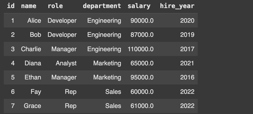
We can first select records from people working in sales, then update their salary, then select them again to show that they’ve changed.
print("Before update:")
results = cursor.execute("SELECT name, salary FROM staff WHERE department = 'Sales';")
display_results(cursor, results)

cursor.execute("""
UPDATE staff
SET salary = salary + 5000
WHERE department = 'Sales' AND role = 'Rep';
""")
conn.commit()

print("\nAfter update:")
results = cursor.execute("SELECT name, salary FROM staff WHERE department = 'Sales';")
display_results(cursor, results)
Both SELECT statements are the same
SELECT name, salary FROM staff WHERE department = 'Sales';but in between we’re using an UPDATE statement to modify the values in the staff table.
UPDATE staff
SET salary = salary + 5000
WHERE department = 'Sales';
Here, for every record in our filtered table, we’re UPDATEing the salary column in each record by SETing it as the salary + 5000. So, everyone in the Sales deparment get’s a 5000 raise!
We can delete people from our staff table using the DELETE keyword.
print("\nBefore delete:")
results = cursor.execute("SELECT name, hire_year FROM staff ORDER BY hire_year;")
display_results(cursor, results)

cursor.execute("""
DELETE FROM staff
WHERE hire_year < 2018;
""")
conn.commit()

print("\nAfter delete:")
results = cursor.execute("SELECT name, hire_year FROM staff ORDER BY hire_year;")
display_results(cursor, results)
We’re almost done with what I would call the intermediate difficulty of SQL. I think one last critical idea we have to discuss is the handling of Null values.
Handling Nulls
Let’s create a table with a bunch of NULL values.
# Create a new database
conn = sqlite3.connect("example_database_12.db")
cursor = conn.cursor()

# Create table and insert data with some NULLs
cursor.executescript("""
DROP TABLE IF EXISTS projects;

CREATE TABLE projects (
    id INTEGER PRIMARY KEY,
    name TEXT,
    manager TEXT,
    budget REAL
);

-- Insert sample data
INSERT INTO projects (name, manager, budget) VALUES
  ('Apollo', 'Alice', 100000),
  ('Beacon', 'Bob', NULL),
  ('Comet', NULL, 75000),
  ('Drift', 'Diana', NULL),
  ('Echo', NULL, NULL);
""")

display_table(cursor, 'projects')
We can get the projects WHERE the manager IS NULL
print("Projects with no assigned manager:")
results = cursor.execute("""

SELECT name
FROM projects
WHERE manager IS NULL;

""")
display_results(cursor, results)
We can get projects with a budget assigned.
print("\nProjects with a budget assigned:")
results = cursor.execute("""

SELECT name, budget
FROM projects
WHERE budget IS NOT NULL;

""")
display_results(cursor, results)
NULL values impact aggregation functions like COUNT and AVG , as one might expect. COUNT(*) counts all rows, even if the rows are NULL , while COUNT(column) counts all the values in a column which are not NULL.
print("\nHow NULLs affect aggregation:")
results = cursor.execute("""

SELECT
  COUNT(*) AS total_projects,
  COUNT(budget) AS with_budget,
  AVG(budget) AS avg_budget
FROM projects;

""")
display_results(cursor, results)
The COALESCE function can be used to replace NULL values within a column, which is pretty handy.
print("Show manager or use 'Unassigned' if NULL:")
results = cursor.execute("""

SELECT name, COALESCE(manager, 'Unassigned') AS display_manager
FROM projects;

""")
display_results(cursor, results)
COALESCE is useful for all sorts of stuff.
print("\nShow budget, default to 0 if missing:")
results = cursor.execute("""

SELECT name, COALESCE(budget, 0) AS safe_budget
FROM projects;

""")
display_results(cursor, results)
Ok, I think we’ve covered most of the fundamentals of SQL. If you stopped here, you would have a working understanding that you could use to do most work in most applications.
Let’s build on this understanding by exploring some more advanced SQL patterns.
Sub-Querying
Lets whip up another database, similar to some of the one’s we’ve used previously.
conn = sqlite3.connect("example_database_13.db")
cursor = conn.cursor()

cursor.executescript("""
DROP TABLE IF EXISTS staff;

CREATE TABLE staff (
    id INTEGER PRIMARY KEY,
    name TEXT,
    role TEXT,
    department TEXT,
    salary REAL,
    hire_year INTEGER
);

INSERT INTO staff (name, role, department, salary, hire_year) VALUES
  ('Alice', 'Developer', 'Engineering', 90000, 2020),
  ('Bob', 'Developer', 'Engineering', 87000, 2019),
  ('Charlie', 'Manager', 'Engineering', 110000, 2017),
  ('Diana', 'Analyst', 'Marketing', 65000, 2021),
  ('Ethan', 'Manager', 'Marketing', 95000, 2016),
  ('Fay', 'Rep', 'Sales', 60000, 2022),
  ('Grace', 'Rep', 'Sales', 61000, 2022),
  ('Henry', 'Manager', 'Sales', 98000, 2018);
""")
“Sub-Querying” allows us to put a query inside another query, which is vital when doing operations that require multiple operations to happen.
For instance, if we wanted to get all of the employees earning more than the average salary, we would need to first get the average salary, then filter by that average salary. We can do that with the following expression:
print("Employees earning more than the average salary:")
results = cursor.execute("""

SELECT name, salary
FROM staff
WHERE salary > (
    SELECT AVG(salary) FROM staff
);

""")

display_results(cursor, results)
In SQL, parenthesis allows us to group a query within another query, so we’re getting the AVG of all salaries, then filtering WHERE salary is greater than that number.
To understand better, we can work through an even more complex example
SELECT name, department
FROM staff
WHERE salary > (
    -- Subquery: Average salary for this person's department
    SELECT AVG(s1.salary)
    FROM staff s1
    WHERE s1.department = staff.department
)
AND department IN (
    -- Departments with above-company-average salary
    SELECT department
    FROM staff
    GROUP BY department
    HAVING AVG(salary) > (
        -- Overall average salary
        SELECT AVG(salary) FROM staff
    )
);
Here, the salary is calculated based on what’s called a “correlated subquery”, which means we’re doing a sub-query based on the values in a row of the top-level query.
We’re evaluating each row in staff with this outer SELECT / WHERE expression
SELECT name, department
FROM staff
WHERE salary > (
...
Then for each row in staff , we’re evaluating this sub query:
-- Subquery: Average salary for this person's department
SELECT AVG(s1.salary)
FROM staff s1
WHERE s1.department = staff.department
Here, we’re renaming staff as s1 within the sub-query, so we’re, conceptually, using two separate copies of staff ; staff and s1.
Within the sub-query, we’re filtering s1 WHERE s1.department = staff.department for the current row of staff , then selecting the AVG of s1.salary from the result. The comparison of s1 and staff is what makes this a correlated subquery.
because there’s no GROUP BY in the sub-query, the result spits out a number. That number get’s re-evaluated for each row, allowing us to compare that number with the salary of the current row.
SELECT name, department
FROM staff
WHERE salary > (
    -- Subquery: Average salary for this person's department
    SELECT AVG(s1.salary)
    FROM staff s1
    WHERE s1.department = staff.department
)
Thus, we’re only preserving the rows where the salary is greater than the average salary in the department the row is from. You might think, wow, that’s really inefficient, however modern SQL engines usually re-write simple correlated sub-queries into a more efficient representation using JOINs and GROUP BYs.
I find correlated subqueries to be both inefficient and counterintuitive, so I don’t really use them, but they’re nifty to know. We’ll explore other, simpler, and more efficient approaches to problems like this in the next section.
In this example, there are two subqueries within the where statement.
-- the second subquery
AND department IN (
    -- Departments with above-company-average salary
    SELECT department
    FROM staff
    GROUP BY department
    HAVING AVG(salary) > (
        -- Overall average salary
        SELECT AVG(salary) FROM staff
    )
);
This one checks if the department has an average salary which is greater than the overall average salary (which is the result of yet another sub-query).
So, the total expression
SELECT name, department
FROM staff
WHERE salary > (
    -- Subquery: Average salary for this person's department
    SELECT AVG(s1.salary)
    FROM staff s1
    WHERE s1.department = staff.department
)
AND department IN (
    -- Departments with above-company-average salary
    SELECT department
    FROM staff
    GROUP BY department
    HAVING AVG(salary) > (
        -- Overall average salary
        SELECT AVG(salary) FROM staff
    )
);
returns the name and department from staff WHERE the salary of each record is greater than the average salary of the department that record is in, AND WHERE the record is IN the list of departments within staff that have a higher than average salary based on all staff members.
This is a lot of logic to wrap into a single expression, which is why the next concept is so useful.
Common Table Expressions
When doing complex sub-querying it can sometimes make sense to define new tables, temporarily, to help you perform a query. That get’s done with the WITH statement and is called a “Common Table Expression”.
print("Complex Expression")

results = cursor.execute("""

WITH
-- 1. Department average salaries
dept_avg AS (
    SELECT department, AVG(salary) AS dept_salary_avg
    FROM staff
    GROUP BY department
),

-- 2. Company-wide average salary
company_avg AS (
    SELECT AVG(salary) AS overall_avg_salary
    FROM staff
),

-- 3. Departments with above-company-average salaries
above_avg_departments AS (
    SELECT d.department
    FROM dept_avg d
    JOIN company_avg c
    WHERE d.dept_salary_avg > c.overall_avg_salary
)

SELECT s.name, s.department
FROM staff s
JOIN dept_avg d ON s.department = d.department
JOIN above_avg_departments a ON s.department = a.department
WHERE s.salary > d.dept_salary_avg;

""")

display_results(cursor, results)
Here, we broke up our complex query with correlated sub-queries into three simple common table expressions, and then used those common table expressions to create our final query.
first, we define a table called dept_avg , which is defined AS the department and AVG(salary) (which is renamed to dept_salary_avg ) from the staff table. The AVG calculation is modified by GROUP BY department.
print("Common Table Expression 1")

results = cursor.execute("""

WITH
-- 1. Department average salaries
dept_avg AS (
    SELECT department, AVG(salary) AS dept_salary_avg
    FROM staff
    GROUP BY department
)

SELECT * FROM dept_avg

""")

display_results(cursor, results)
The second common table expression simply calculates the average salary of all staff, and renames it as a column called overall_avg_salary which is within a table called company_avg.
print("Common Table Expression 2")

results = cursor.execute("""

WITH
company_avg AS (
    SELECT AVG(salary) AS overall_avg_salary
    FROM staff
)

SELECT * from company_avg

""")

display_results(cursor, results)
The final common table expression defines a table called above_avg_departments which uses the two previous common table expressions to find departments whos average salary is greater than the overall average.
print("Complex Expression")

results = cursor.execute("""

WITH
-- 1. Department average salaries
dept_avg AS (
    SELECT department, AVG(salary) AS dept_salary_avg
    FROM staff
    GROUP BY department
),

-- 2. Company-wide average salary
company_avg AS (
    SELECT AVG(salary) AS overall_avg_salary
    FROM staff
),

-- 3. Departments with above-company-average salaries
above_avg_departments AS (
    SELECT d.department
    FROM dept_avg d
    JOIN company_avg c
    WHERE d.dept_salary_avg > c.overall_avg_salary
)

SELECT * from above_avg_departments

""")

display_results(cursor, results)
This works because when you call JOIN on a single-row table, the row is automatically broadcast to all rows. So, we’re broadcasting the single, row table company_avg over all rows of dept_avg , then keeping all rows WHERE the dept_avg.dept_salary_avg is greater than the company_avg.overall_avg_salary .
Using all those tables, the final expression finds all people who have a higher than average salary in their respective department, where that department has a higher than average salary relative to all salaries.
print("Complex Expression")

results = cursor.execute("""

WITH
-- 1. Department average salaries
dept_avg AS (
    SELECT department, AVG(salary) AS dept_salary_avg
    FROM staff
    GROUP BY department
),

-- 2. Company-wide average salary
company_avg AS (
    SELECT AVG(salary) AS overall_avg_salary
    FROM staff
),

-- 3. Departments with above-company-average salaries
above_avg_departments AS (
    SELECT d.department
    FROM dept_avg d
    JOIN company_avg c
    WHERE d.dept_salary_avg > c.overall_avg_salary
)

SELECT s.name, s.department
FROM staff s
JOIN dept_avg d ON s.department = d.department
JOIN above_avg_departments a ON s.department = a.department
WHERE s.salary > d.dept_salary_avg;

""")

display_results(cursor, results)
We can peek behind the scenes a bit by using SELECT * and removing the WHERE statement to get an idea of what the final table looks like.
print("Complex Expression")

results = cursor.execute("""

WITH
-- 1. Department average salaries
dept_avg AS (
    SELECT department, AVG(salary) AS dept_salary_avg
    FROM staff
    GROUP BY department
),

-- 2. Company-wide average salary
company_avg AS (
    SELECT AVG(salary) AS overall_avg_salary
    FROM staff
),

-- 3. Departments with above-company-average salaries
above_avg_departments AS (
    SELECT d.department
    FROM dept_avg d
    JOIN company_avg c
    WHERE d.dept_salary_avg > c.overall_avg_salary
)

SELECT *
FROM staff s
JOIN dept_avg d ON s.department = d.department
JOIN above_avg_departments a ON s.department = a.department

""")

display_results(cursor, results)
The expression
JOIN dept_avg d ON s.department = d.departmentjoins our staff to our dept_avg table, getting us the dept_salary_avg column.
For the next JOINexpression, because it’s a JOIN expression, (and not a LEFT JOIN , RIGHT JOIN , or OUTER JOIN ) we only keep rows which have values in both tables. So, the expression
JOIN above_avg_departments a ON s.department = a.departmentonly preserves rows where the staff.department is equal to the above_avg_departments.department . The only one of those is Engineering , so that’s why this table only has Engineering people. If they’ve made it this far in the tutorial, they’ve earned it.
Then, we simply SELECT whatever columns we want, like the name and the department, and filter WHERE the salary is greater than the dept_salary_avg for a particular row.
SELECT s.name, s.department
FROM staff s
JOIN dept_avg d ON s.department = d.department
JOIN above_avg_departments a ON s.department = a.department
WHERE s.salary > d.dept_salary_avg;
Recursive Common Table Expressions
If you’ve gotten to this point, you probably have an idea of what recursion is in general. It’s when a function calls itself based on the output of the previous iteration. SQL has a similar concept of recursion.
# No table needed — it's a pure CTE demo

print("Generating numbers 1 to 10 using a recursive CTE:")

results = cursor.execute("""
WITH RECURSIVE numbers(n) AS (
    SELECT 1               -- Base case
    UNION ALL
    SELECT n + 1           -- Recursive case
    FROM numbers
    WHERE n < 10           -- Stopping condition
)
SELECT * FROM numbers;
""")

display_results(cursor, results)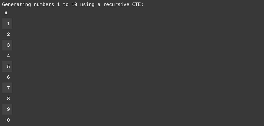
When defining a new table via a common table expression, you can specify column names with the syntax:
WITH my_cte(col1, col2) AS (
    ...
)
where my_cte is the name of the table and col1 and col2 are columns. So, in this block of SQL, we’re creating a table numbers with a single column n.
When defining a recursive CTE, there are three fundamental steps:
The base case (defining the initial set of rows), which is defined with
SELECTUNION ALL, which combines all outputs of recursionAnother
SELECT, which defines the recursion selection.
a RECURSIVE common table expression keeps running the recursive SELECT untill it outputs an empty table. Commonly, this is achieved with a WHERE clause within the recursive SELECT statement, but it doesn’t necessarily have to have it.
The thing that makes this “Recursion”, and not just a loop, is that the result of the recursion selection is passed as the input into the next round of recursion selection.
So, we initialize our recursive common table with:
WITH RECURSIVE numbers(n) AS (
    SELECT 1               -- Base case
...
resulting in a base table like this:
numbers
--------
n
1
Then, we combine to that table some set of tables:
WITH RECURSIVE numbers(n) AS (
    SELECT 1               -- Base case
    UNION ALL
...
Which are defined by this recursive selection, which runs over and over untill it outputs an empty table.
WITH RECURSIVE numbers(n) AS (
    SELECT 1               -- Base case
    UNION ALL
    SELECT n + 1           -- Recursive case
    FROM numbers
    WHERE n < 10           -- Stopping condition
)
The first round of recursive selection takes in our base table
numbers
--------
n
1
and applies the query
SELECT n + 1
FROM numbers
WHERE n < 10
when you do SELECT column + value , SQL adds the value to every row in the column. Because our base table just has one value, we get the result
numbers
--------
n
2
So, that’s the result of our first iteration.
That result gets passed as the input for our second round of recursive iteration
SELECT n + 1
FROM numbers
WHERE n < 10
which results in
numbers
--------
n
3
etc.
when the input to the recursive SELECT clause is
numbers
--------
n
10
the WHERE clause filters out out all rows, resulting in an empty row. When an empty row is returned, the recursive common table expression is terminated.
So, now we have a big list of tables, output from various iterations of the recursive select statement, along with the base case.
numbers (base case)
--------
n
1

numbers (iteration 1)
--------
n
2

numbers (iteration 2)
--------
n
3

numbers (iteration 3)
--------
n
4
...
the UNION ALL expression declares that we want all of the iterations combined with our base case, resulting in our final output:
numbers
--------
n
1
2
3
4
5
6
7
8
9
10
Recursive common table expressions are particularly useful when analyzing hierarchical data. Imagine we had some organization where certain people are managed by other people.
conn = sqlite3.connect("example_database_15.db")
cursor = conn.cursor()

cursor.executescript("""
DROP TABLE IF EXISTS employees;

CREATE TABLE employees (
    id INTEGER PRIMARY KEY,
    name TEXT,
    title TEXT,
    manager_id INTEGER,
    FOREIGN KEY (manager_id) REFERENCES employees(id)
);

INSERT INTO employees (id, name, title, manager_id) VALUES
  (1, 'Henry', 'CEO', NULL),
  (2, 'Alice', 'CTO', 1),
  (3, 'Diana', 'CFO', 1),
  (4, 'Bob', 'Engineer', 2),
  (5, 'Cara', 'Engineer', 2),
  (6, 'Ella', 'Accountant', 3);
""")
Here, Henry is the CEO and isn’t managed by anyone. Henry manages ALice amd Diana who in tern manage Bob, Cara, and Ella.
If we wanted to calculate the level of each person in the hierarchy, we could use the following recursive common table expression:
print("Organizational hierarchy:")

results = cursor.execute("""
WITH RECURSIVE org_chart(id, name, title, manager_id, level) AS (
    -- Base case: start with the CEO
    SELECT id, name, title, manager_id, 0
    FROM employees
    WHERE manager_id IS NULL

    UNION ALL

    -- Recursive step: find employees reporting to those already found
    SELECT e.id, e.name, e.title, e.manager_id, oc.level + 1
    FROM employees e
    JOIN org_chart oc ON e.manager_id = oc.id
)
SELECT name, title, level
FROM org_chart
ORDER BY level, name;
""")

display_results(cursor, results)
Here, the base case is Henry, the CEO, and we define their level initially as level 0.
id | name  | title | manager_id | level
---+-------+-------+------------+------
1  | Henry | CEO   | NULL       | 0
That base case is the input for our first recursive iteration.
from that base case, we call the expression
SELECT e.id, e.name, e.title, e.manager_id, oc.level + 1
FROM employees e
JOIN org_chart oc ON e.manager_id = oc.id
Where we’re renaming the entire original eomployees table as e, and the result of recursive iteration org_chart as oc. Using those two table, we join the orc_chart(oc) onto employees(e) where e.manager_id = oc.id. Because this is a JOIN (and not a left or full outer join) we only preserve rows where there is a value that satisfies e.manager_id = oc.id . Practically, for this first iteration, that means we’re preserving only the employees who are managed by Henry, and combining Henry’s information onto the table.
The SELECT statement then filters down the columns of the table to the new employees e.id, e.name, e.title, e.manager_id , but keeps Henry’s level, but adds 1 to it. The result is the following:
id | name  | title | manager_id | level
---+-------+-------+------------+------
2  | Alice | CTO   | 1          | 1
3  | Diana | CFO   | 1          | 1
That’s the result of the first round of recursion, and the input to the second round of recursion.
So, we JOIN this instance of org_chart onto the employees table based on the relationship of manager_id with id, resulting in a new table with all of the people being managed, and their manager. We preserve the people being managed, and their manager’s value + 1, resulting in the next round of iteration.
id | name  | title      | manager_id | level
---+-------+------------+------------+------
4  | Bob   | Engineer   | 2          | 2
5  | Cara  | Engineer   | 2          | 2
6  | Ella  | Accountant | 3          | 2
Passing this to the final recursive loop, the JOIN expression results in an empty output, as these people don’t manage anyone, triggering the end of recursion.
All of these result tables are combined with the base case, resulting in the following output:
name   | title      | level
-------+------------+------
Henry  | CEO        | 0
Alice  | CTO        | 1
Diana  | CFO        | 1
Bob    | Engineer   | 2
Cara   | Engineer   | 2
Ella   | Accountant | 2
Hopefully this is starting to make sense, let’s go through one more recursive example to lock in the idea.
So, same table, but imagine we want to print out the hierarchy of each person who has a manager, in conjunction with their title.

To do that, we can use yet another recursive common table expression.
print("Flattened reporting chains with titles:")

results = cursor.execute("""
WITH RECURSIVE org_paths(id, name, title, manager_id, path) AS (
    -- Base case: CEO
    SELECT id, name, title, manager_id, name
    FROM employees
    WHERE manager_id IS NULL

    UNION ALL

    -- Recursive step: extend the path
    SELECT e.id, e.name, e.title, e.manager_id, op.path || ' > ' || e.name
    FROM employees e
    JOIN org_paths op ON e.manager_id = op.id
)
SELECT path || ' (' || title || ')' AS full_path
FROM org_paths
WHERE id != 1
ORDER BY path;
""")

display_results(cursor, results)
So, the base case is all people where the manager_id is NULL , which is only the CEO in this case. Here, we’re defining the column names of org_paths as (id, name, title, manager_id, path) and, for this first round, we’re setting the path as just the name
-- Base case: CEO
SELECT id, name, title, manager_id, name
FROM employees
WHERE manager_id IS NULL
id | name | title | manager_id | path
---+-------+-------+------------+-----
1 | Henry | CEO | NULL | HenryThat base case is the input, named org_paths, for the first round of iteration.
Then, we’re doing a similar trick as the previous example. We’re joining org_paths onto the whole employees table.
Instead of specifying the path as just the name, we’re specifying the path as op.path || ‘ > ‘ || e.name , where op is a pseudonym for org_paths and e is a pseudonym for employees. In SQL, || means string concatenation, so combining strings together, so we’re combining the path of the manager with the name of the employee to define the path for the employee.
For the first recursive output, we get:
id | name  | title | manager_id | path
---+-------+-------+------------+--------------------
2  | Alice | CTO   | 1          | Henry > Alice
3  | Diana | CFO   | 1          | Henry > Diana
That’s the input for the second round of recursion, which results in:
id | name  | title      | manager_id | path
---+-------+------------+------------+--------------------------
4  | Bob   | Engineer   | 2          | Henry > Alice > Bob
5  | Cara  | Engineer   | 2          | Henry > Alice > Cara
6  | Ella  | Accountant | 3          | Henry > Diana > Ella
the next round of recursion results in an empty table, ending the recursive loop.
All recursive outputs are concatenated together, and is used to trigger the final SELECT clause
SELECT path || ' (' || title || ')' AS full_path
FROM org_paths
WHERE id != 1
ORDER BY path;
Here we’re outputting the final table as a single column called full_path , which is the string concatenation of the path with the persons title encased in parentheses. We’re also not returning id = 1 , which is the CEO.
We’re using ORDER BY path to sort the paths by alphabetical order. And, thus, we get our final output:
Window Functions
Imagine you have the following table:
conn = sqlite3.connect("example_database_16.db")
cursor = conn.cursor()

cursor.executescript("""
DROP TABLE IF EXISTS sales;

CREATE TABLE sales (
    id INTEGER PRIMARY KEY,
    employee TEXT,
    department TEXT,
    amount REAL
);

INSERT INTO sales (employee, department, amount) VALUES
  ('Alice', 'Engineering', 1000),
  ('Bob', 'Engineering', 1500),
  ('Joe', 'Engineering', 1500),
  ('Charlie', 'Engineering', 1200),
  ('Diana', 'Marketing', 800),
  ('Ethan', 'Marketing', 700),
  ('Fay', 'Sales', 900),
  ('Grace', 'Sales', 1300);
""")
Each employee in the sales table has an amount they’ve sold, and belong to a specific department. If we wanted to rank everyone based on their department, we could use a window function.
SELECT employee, department, amount,
       ROW_NUMBER() OVER (PARTITION BY department ORDER BY amount DESC) AS row_num
FROM sales;
Here ROW_NUMBER is a window function which operates OVER rows in a database. PARTITION BY is an optional keyword inside OVER which allows you to divide the table into sections each of which to uniquely have a window function applied. So, we’re partioning our table by department, ORDERing each of those partitions by the sale amount in descending order, and then counting each row. The result of doing that counting is called row_num .
That’s all happening within the SELECT statement, so row_num gets returned along with employee, department, amount from the sales table.

There are many window functions in SQL. For instance, Joe might be upset that he’s ranked under Bob, so we can use the RANK window function instead of using ROW_NUMBER to count rows.
print("Scoreboard:")

results = cursor.execute("""

SELECT employee, department, amount,
       RANK() OVER (PARTITION BY department ORDER BY amount DESC) AS rank,
       DENSE_RANK() OVER (PARTITION BY department ORDER BY amount DESC) AS dense_rank
FROM sales;


""")

display_results(cursor, results)
Here, we’re using two different flavors of ranking, RANK and DENSE_RANK , both of which handle the rank after a tie differently.
These functions know which column to calculate rank based off of because of the ORDER BY amount statement. Because we’re ordering by amount, the RANK window function automatically knows to calculate rank by amount. If we didn’t specify an ORDER BY , the RANK function wouldn’t know what to calculate rank based off of
print("Scoreboard:")

results = cursor.execute("""

SELECT employee, department, amount,
       RANK() OVER (PARTITION BY department) AS rank
FROM sales;


""")

display_results(cursor, results)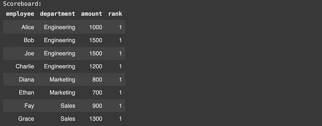
Some window functions don’t need order. For instance, the SUM function just needs a window to play with
print("Scoreboard:")

results = cursor.execute("""

SELECT employee, department, amount,
       SUM(amount) OVER (PARTITION BY department) AS department_total,
       SUM(amount) OVER () AS department_total
FROM sales;


""")

display_results(cursor, results)
Here I’m calculating the SUM over each partition, and also I’m calculating the total SUM. I’m telling the SUM function which column to aggregate by by specifying the column name in the argument of the function. I’m calculating the second SUM OVER () because the existence of parentheses is required when specifying a window function, which return an output for each value. If I just did SUM(amount) AS department_total, it would cause the table to collapse to a single value, which isn’t what we want in this example.
print("Scoreboard:")

results = cursor.execute("""

SELECT employee, department, amount,
       SUM(amount) OVER (PARTITION BY department) AS department_total,
       SUM(amount) AS department_total
FROM sales;


""")

display_results(cursor, results)
There are a ton of window functions to choose from in SQL. There are window functions based on ranking and row position:
ROW_NUMBER()Unique row number per partition/orderRANK()Rank with gaps for tiesDENSE_RANK()Rank without gaps for tiesNTILE(n)Divides rows intonbuckets
window functions for looking back/ahead
LAG(column, offset, default)Value from a previous rowLEAD(column, offset, default)Value from a future rowFIRST_VALUE(column)First value in the windowLAST_VALUE(column)Last value in the windowNTH_VALUE(column, n)nth value in the window
aggregate style window functions, that when used in a window function broadcast their aggregation to all rows
SUM()Sum of values in the windowAVG()Average of values in the windowCOUNT()Count of rows in the windowMIN()Minimum value in the windowMAX()Maximum value in the window
There’s constrain window functions to not cover the entire partition, but a subset around the particular value in which the window function is defined. Here’s an example of a moving average, for instance.
SELECT
  employee,
  amount,
  AVG(amount) OVER (
    ORDER BY ammount
    ROWS BETWEEN 1 PRECEDING AND 1 FOLLOWING
  ) AS moving_avg
FROM sales;
SQL is dense, and there’s, frankly, too much to learn. The important part is to know what’s possible so you can google when needed.
You can check out the full code for a few more examples of window functions.
There are a ton more topics to cover, like pivot tables, upsets, permissions and security, date and time functions… SQL has been around for a while, and there is a ton of stuff to know. For now, though, I think we’ve created a solid working understanding where, if we don’t know something, we can figure it out with a bit of research.
Let’s go through a few crazy SQL examples and work through them line-by-line to galvanize our understanding.
Have any questions about this article? Join the IAEE Discord.
Crazy Example 1
Setting up the database
import sqlite3

conn = sqlite3.connect("example_database_19.db")
cursor = conn.cursor()

cursor.executescript("""
DROP TABLE IF EXISTS students;
DROP TABLE IF EXISTS courses;
DROP TABLE IF EXISTS enrollments;
DROP TABLE IF EXISTS prerequisites;

CREATE TABLE students (
    id INTEGER PRIMARY KEY,
    name TEXT
);

CREATE TABLE courses (
    id INTEGER PRIMARY KEY,
    course_name TEXT
);

CREATE TABLE enrollments (
    student_id INTEGER,
    course_id INTEGER,
    grade INTEGER,  -- out of 100
    FOREIGN KEY (student_id) REFERENCES students(id),
    FOREIGN KEY (course_id) REFERENCES courses(id)
);

CREATE TABLE prerequisites (
    course_id INTEGER,
    prerequisite_id INTEGER,
    FOREIGN KEY (course_id) REFERENCES courses(id),
    FOREIGN KEY (prerequisite_id) REFERENCES courses(id)
);

-- Students
INSERT INTO students (id, name) VALUES
  (1, 'Alice'),
  (2, 'Bob'),
  (3, 'Cara');

-- Courses
INSERT INTO courses (id, course_name) VALUES
  (1, 'Math'),
  (2, 'History'),
  (3, 'Science'),
  (4, 'Advanced Science');

-- Enrollments (with grades)
INSERT INTO enrollments (student_id, course_id, grade) VALUES
  (1, 1, 95),  -- Alice - Math
  (1, 2, 80),
  (1, 3, 88),
  (1, 4, 91),  -- Took Advanced

  (2, 1, 75),
  (2, 3, 82),
  (2, 4, 85),  -- Took Advanced, skipped History

  (3, 1, 100),
  (3, 2, 85),
  (3, 3, 80);  -- Did not take Advanced

-- Prerequisites (Advanced Science requires Science)
INSERT INTO prerequisites (course_id, prerequisite_id) VALUES
  (4, 3);
""")
there’s a table for students , courses , enrollments , and prerequisites. We then populate those tables with some mock data.
Based on this table, let’s specify an SQL expression that produces a table that expresses the following:
Each row in the table represents a student’s performance in one specific course, but only if the student has completed all the necessary prerequisites for that course.
For each of those student-course pairs, the table shows:
student The name of the student
course_name The name of the course they took
grade The score they received in that course (out of 100)
rank_in_course Their rank in the class for that course (1 = top scorer, 2 = second-highest, etc.)
relative_score Their grade as a percentage of the top score in the class — e.g., “95.0%” means they got 95% of the top grade
top_marker A label that shows ✅ “Top of Class” if they had the highest grade in the course, or blank otherwise
total_courses The total number of courses the student has taken overall
avg_grade The student’s average grade across all courses they’ve taken
If a student took a course without completing all of its prerequisites, that student will not appear at all in the final table.
That SQL expression looks like the following:
print("Crazy complex query mixing everything:")

results = cursor.execute("""
WITH RECURSIVE prereq_chain(course_id, prerequisite_id) AS (
    -- Base case: start with prerequisites
    SELECT course_id, prerequisite_id
    FROM prerequisites
    UNION
    -- Recursively walk the tree of prerequisites
    SELECT p.course_id, pr.prerequisite_id
    FROM prerequisites p
    JOIN prereq_chain pr ON p.prerequisite_id = pr.course_id
),

-- Who took what
student_courses AS (
    SELECT student_id, course_id, grade
    FROM enrollments
),

-- Build course stats (ranking and percent)
course_ranking AS (
    SELECT
        e.student_id,
        c.course_name,
        e.course_id,
        e.grade,
        RANK() OVER (PARTITION BY e.course_id ORDER BY e.grade DESC) AS rank_in_course,
        ROUND(100.0 * e.grade / MAX(e.grade) OVER (PARTITION BY e.course_id), 2) AS pct_of_top,
        CASE WHEN e.grade = MAX(e.grade) OVER (PARTITION BY e.course_id)
             THEN '✅ Top of Class'
             ELSE ''
        END AS top_marker
    FROM enrollments e
    JOIN courses c ON c.id = e.course_id
),

-- Check who is missing prerequisites
missing_prereqs AS (
    SELECT DISTINCT sc.student_id, pc.course_id
    FROM prereq_chain pc
    JOIN student_courses sc ON sc.course_id = pc.course_id
    WHERE NOT EXISTS (
        SELECT 1
        FROM student_courses inner_sc
        WHERE inner_sc.student_id = sc.student_id
          AND inner_sc.course_id = pc.prerequisite_id
    )
)

-- Final selection
SELECT
    s.name AS student,
    cr.course_name,
    cr.grade,
    cr.rank_in_course,
    cr.pct_of_top || '%' AS relative_score,
    cr.top_marker,
    (
      SELECT COUNT(*) FROM enrollments e WHERE e.student_id = s.id
    ) AS total_courses,
    (
      SELECT ROUND(AVG(grade), 1) FROM enrollments e WHERE e.student_id = s.id
    ) AS avg_grade
FROM course_ranking cr
JOIN students s ON s.id = cr.student_id
WHERE cr.student_id NOT IN (
    SELECT student_id FROM missing_prereqs
)
ORDER BY s.name, cr.course_id;
""")

display_results(cursor, results)
To make this problem more manageable, common table expressions are used to subdivide the problem into smaller problems.
prereq_chain is used to calculate all prerequisites, including indirect ones. For instance, if class 1 is a prereq for class 2, and class 2 is a prereq for class 3, then class 1 is a prereq for class 3 in the prereq_chain.
WITH RECURSIVE prereq_chain(course_id, prerequisite_id) AS (
    -- Base case: start with prerequisites
    SELECT course_id, prerequisite_id
    FROM prerequisites
    UNION
    -- Recursively walk the tree of prerequisites
    SELECT p.course_id, pr.prerequisite_id
    FROM prerequisites p
    JOIN prereq_chain pr ON p.prerequisite_id = pr.course_id
),
We do that calculation by establishing the direct prerequisites as a base case
SELECT course_id, prerequisite_id
FROM prerequisites
Then we recursively walk through the prerequisites of those prerequisites
SELECT p.course_id, pr.prerequisite_id
FROM prerequisites p
JOIN prereq_chain pr ON p.prerequisite_id = pr.course_id
Once we run out of classes that are pre-requisites of pre-requisites of pre-requisites, etc. we union all those tables to create an exhaustive table of classes and all of their derivative prerequisites.
We also create a common table expression that helps us keep track of who took what class. This might be kind of redundant, because it doesn’t really do anything, but it helps for organizational purposes and an SQL engine can easily optimize this to not impact search performance.
student_courses AS (
    SELECT student_id, course_id, grade
    FROM enrollments
),
We create another common table expression that has rank information
-- Build course stats (ranking and percent)
course_ranking AS (
    SELECT
        e.student_id,
        c.course_name,
        e.course_id,
        e.grade,
        RANK() OVER (PARTITION BY e.course_id ORDER BY e.grade DESC) AS rank_in_course,
        ROUND(100.0 * e.grade / MAX(e.grade) OVER (PARTITION BY e.course_id), 2) AS pct_of_top,
        CASE WHEN e.grade = MAX(e.grade) OVER (PARTITION BY e.course_id)
             THEN '✅ Top of Class'
             ELSE ''
        END AS top_marker
    FROM enrollments e
    JOIN courses c ON c.id = e.course_id
),
this runs a JOIN between enrollments and courses , meaning courses without enrollments get dropped, and enrollments without courses get dropped. We then SELECT basic information like the student_id , course_name , course_id , and grade.
We calculate the rank of each student of each class using the RANK() window function OVER the rows, PARTITIONED BY the course_id and ORDER BY the grades of the students in that course.
In a slightly different manner to previous window functions we’ve discussed, we calculate the pct_of_top by calculating the percentage of each grade relative to the MAX of all grades for a particular course_id
100.0 * e.grade / MAX(e.grade) OVER (PARTITION BY e.course_id)That is wrapped within a ROUND functions, which rounds all of the values in the expression. this function specifies that we’re rounding to two decimal places.
ROUND(100.0 * e.grade / MAX(e.grade) OVER (PARTITION BY e.course_id), 2)Finally, in another thing we haven’t seen before, we’re using a CASE clause to make a decision as to whether to render ‘✅ Top of Class’ for a particular record. This is defined as a window function via the following:
CASE WHEN e.grade = MAX(e.grade) OVER (PARTITION BY e.course_id)
  THEN '✅ Top of Class'
  ELSE ''
END AS top_marker
CASE expressions obey the following general form:
CASE
  WHEN condition1 THEN result1
  WHEN condition2 THEN result2
  ELSE fallback_result
END
So, when the condition e.grade = MAX(e.grade) is true, across the window which is defined by OVER (PARTITION BY e.course_id) , then the value of that row in the window has a value of ‘✅ Top of Class’ as top_marker.
We employ one more common table expression, to keep track of students who do not have all their prerequisites.
-- Check who is missing prerequisites
missing_prereqs AS (
    SELECT DISTINCT sc.student_id, pc.course_id
    FROM prereq_chain pc
    JOIN student_courses sc ON sc.course_id = pc.course_id
    WHERE NOT EXISTS (
        SELECT 1
        FROM student_courses inner_sc
        WHERE inner_sc.student_id = sc.student_id
          AND inner_sc.course_id = pc.prerequisite_id
    )
)
Here, we’re joining the two previously defined common table expressions, student_courses and prereq_chainon course_id , meaning we’re joining based on if the course id of a student matches the the course. Before this point,
prereq_chainhas the columnscourse_idandprerequisite_id, and lists out all of the combinations of courses and their prereques (not just immediate ones).student_coursesis just a table of which classes each student is taking. it has the columnsstudent_id, course_id, grade
If we just run the join and print out the result, we see a table that looks like this:
-- Check who is missing prerequisites
missing_prereqs AS (
    SELECT DISTINCT *
    FROM prereq_chain pc
    JOIN student_courses sc ON sc.course_id = pc.course_id
)
The bulk of the logic for checking if anyone has a missing prerequisite comes from the WHERE clause. This is a subquery, meaning it gets executed on a per-row basis of the outer query.
-- Check who is missing prerequisites
missing_prereqs AS (
    SELECT DISTINCT sc.student_id, pc.course_id
    FROM prereq_chain pc
    JOIN student_courses sc ON sc.course_id = pc.course_id
    WHERE NOT EXISTS (
        SELECT 1
        FROM student_courses inner_sc
        WHERE inner_sc.student_id = sc.student_id
          AND inner_sc.course_id = pc.prerequisite_id
    )
)
So, on a particular row of the joined sc and pc table, we grab the student_id and prerequisite_id. If the student_courses table (pseudonymed as inner_sc) contains an example, then we SELECT 1. The value in SELECT doesn’t matter, it could be SELECT * , SELECT 42 , whatever. We just want to create a table that contains instances of the student taking the prerequisite of the row specified in the JOIN of student_courses and prereq_chain.
WHERE NOT EXISTS means, on a particular row of that JOIN, if the student has no examples of taking that pre-requisite, then the row will be preserved.
Thus, we will have a record of all of the student_id, course_id pairs where a student did not take the valid prerequisites.
The final query is fairly straight forward, it simply combines these common table expressions and uses them to output the final query.
-- Final selection
SELECT
    s.name AS student,
    cr.course_name,
    cr.grade,
    cr.rank_in_course,
    cr.pct_of_top || '%' AS relative_score,
    cr.top_marker,
    (
      SELECT COUNT(*) FROM enrollments e WHERE e.student_id = s.id
    ) AS total_courses,
    (
      SELECT ROUND(AVG(grade), 1) FROM enrollments e WHERE e.student_id = s.id
    ) AS avg_grade
FROM course_ranking cr
JOIN students s ON s.id = cr.student_id
WHERE cr.student_id NOT IN (
    SELECT student_id FROM missing_prereqs
)
ORDER BY s.name, cr.course_id;
There are a few specifics in the final query, but it’s pretty straight forward.
First of all, we’re joining our course_ranking table with our students table
FROM course_ranking cr
JOIN students s ON s.id = cr.student_id
We’re using string concatenation to put a % symbol on the relatice score, and we actually rename it to relative_score.
cr.pct_of_top || '%' AS relative_scoreWe create a subquery which counts the number of courses a student was enrolled in, for each student id in the outer query.
(
  SELECT COUNT(*) FROM enrollments e WHERE e.student_id = s.id
) AS total_courses,
We calculate the average grade for each student, and broadcast those results across all of the students rows.
(
  SELECT ROUND(AVG(grade), 1) FROM enrollments e WHERE e.student_id = s.id
) AS avg_grade
We only preserve the rows where a student/class combo does not exist in our record of missing prerequisites.
WHERE cr.student_id NOT IN (
    SELECT student_id FROM missing_prereqs
)
And we order by student, then class.
ORDER BY s.name, cr.course_id;Crazy Example 2
Imagine we have some stock data
import sqlite3
from datetime import datetime, timedelta

conn = sqlite3.connect("example_database_20.db")
cursor = conn.cursor()

cursor.executescript("""
DROP TABLE IF EXISTS trades;

CREATE TABLE trades (
    id INTEGER PRIMARY KEY,
    symbol TEXT,
    trade_time TEXT,  -- ISO timestamp
    price REAL,
    volume INTEGER
);
""")

# Generate synthetic data for one symbol over 10 minutes
symbol = 'AAPL'
base_time = datetime(2023, 1, 1, 9, 30)

for i in range(60):
    trade_time = (base_time + timedelta(minutes=i)).strftime('%Y-%m-%d %H:%M:%S')
    price = 150 + (i % 10) * 0.5 + (-1)**i * (i % 3) * 0.2  # wavy pattern
    volume = 100 + (i % 5) * 30 + (i % 2) * 20
    cursor.execute("INSERT INTO trades (symbol, trade_time, price, volume) VALUES (?, ?, ?, ?)",
                   (symbol, trade_time, round(price, 2), volume))

conn.commit()
The following query
Filters trades to only include those for the symbol
'AAPL'.Calculates the previous and next price for each trade using window functions.
Computes a 5-trade moving average of the price.
Calculates the percent return compared to the previous trade.
Labels each trade as trending ↑ UP, ↓ DOWN, or → FLAT based on price change.
Flags trades with unusually high volume compared to the recent average as “⚠️ VOLUME SPIKE”.
Detects and marks local price peaks and dips as “🔺 LOCAL PEAK” or “🔻 LOCAL DIP”
Groups trades by minute and identifies the 15 most active minutes based on total trade volume.
Filters the output to include only trades that occurred during those 15 most active minutes.
Returns a sorted list of these trades with annotated trend, return %, moving average, volume alert, and local extrema.
print("Crazy stock time series analytics:")

results = cursor.execute("""
WITH base AS (
    SELECT *
    FROM trades
    WHERE symbol = 'AAPL'
),

windowed AS (
    SELECT
        id,
        trade_time,
        price,
        volume,
        LAG(price) OVER (ORDER BY trade_time) AS prev_price,
        LEAD(price) OVER (ORDER BY trade_time) AS next_price,
        ROUND(AVG(price) OVER (ORDER BY trade_time ROWS BETWEEN 4 PRECEDING AND CURRENT ROW), 2) AS price_avg_5,
        ROUND(100.0 * (price - LAG(price) OVER (ORDER BY trade_time)) / LAG(price) OVER (ORDER BY trade_time), 2) AS return_pct,
        CASE
            WHEN price > LAG(price) OVER (ORDER BY trade_time) THEN '↑ UP'
            WHEN price < LAG(price) OVER (ORDER BY trade_time) THEN '↓ DOWN'
            ELSE '→ FLAT'
        END AS trend,
        CASE
            WHEN volume > AVG(volume) OVER (ORDER BY trade_time ROWS BETWEEN 4 PRECEDING AND CURRENT ROW) * 1.5 THEN '⚠️ VOLUME SPIKE'
            ELSE ''
        END AS volume_alert,
        CASE
            WHEN price > LAG(price) OVER (ORDER BY trade_time) AND price > LEAD(price) OVER (ORDER BY trade_time) THEN '🔺 LOCAL PEAK'
            WHEN price < LAG(price) OVER (ORDER BY trade_time) AND price < LEAD(price) OVER (ORDER BY trade_time) THEN '🔻 LOCAL DIP'
            ELSE ''
        END AS local_extreme
    FROM base
),

active_window AS (
    SELECT trade_time
    FROM windowed
    GROUP BY strftime('%H:%M', trade_time)
    ORDER BY SUM(volume) DESC
    LIMIT 15
)

SELECT w.trade_time, w.price, w.volume,
       w.trend, w.return_pct || '%' AS return,
       w.price_avg_5 AS "5ma",
       w.volume_alert, w.local_extreme
FROM windowed w
WHERE strftime('%H:%M', w.trade_time) IN (SELECT strftime('%H:%M', trade_time) FROM active_window)
ORDER BY w.trade_time;
""")

display_results(cursor, results)
First of all, our data could have more data than just AAPL, in theory, so we can create a common table expression that only gets out AAPL data
WITH base AS (
    SELECT *
    FROM trades
    WHERE symbol = 'AAPL'
),
There is then a bunch of window based data, which is pretty common in stock price analysis.
windowed AS (
    SELECT
        id,
        trade_time,
        price,
        volume,
        LAG(price) OVER (ORDER BY trade_time) AS prev_price,
        LEAD(price) OVER (ORDER BY trade_time) AS next_price,
        ROUND(AVG(price) OVER (ORDER BY trade_time ROWS BETWEEN 4 PRECEDING AND CURRENT ROW), 2) AS price_avg_5,
        ROUND(100.0 * (price - LAG(price) OVER (ORDER BY trade_time)) / LAG(price) OVER (ORDER BY trade_time), 2) AS return_pct,
        CASE
            WHEN price > LAG(price) OVER (ORDER BY trade_time) THEN '↑ UP'
            WHEN price < LAG(price) OVER (ORDER BY trade_time) THEN '↓ DOWN'
            ELSE '→ FLAT'
        END AS trend,
        CASE
            WHEN volume > AVG(volume) OVER (ORDER BY trade_time ROWS BETWEEN 4 PRECEDING AND CURRENT ROW) * 1.5 THEN '⚠️ VOLUME SPIKE'
            ELSE ''
        END AS volume_alert,
        CASE
            WHEN price > LAG(price) OVER (ORDER BY trade_time) AND price > LEAD(price) OVER (ORDER BY trade_time) THEN '🔺 LOCAL PEAK'
            WHEN price < LAG(price) OVER (ORDER BY trade_time) AND price < LEAD(price) OVER (ORDER BY trade_time) THEN '🔻 LOCAL DIP'
            ELSE ''
        END AS local_extreme
    FROM base
),
There’s really not much crazy going on here. from base, which is our trade data only based on AAPL, we select a few key values.
id, trade_time, price, volume,we get the price LEAD and LAG based on trade_time
LAG(price) OVER (ORDER BY trade_time) AS prev_price,
LEAD(price) OVER (ORDER BY trade_time) AS next_price,
we also calculate a moving average, which is the average of the value and five preceding values for every timestep
ROUND(AVG(price)
OVER(
  ORDER BY trade_time
  ROWS BETWEEN 4 PRECEDING AND CURRENT ROW),
2) AS price_avg_5,
We specify the 5 timesteps as the 4 PRECEDING AND CURRENT ROW within the window function. That also gets rounded to two decimal places.
This expression calculates the percent return from the previous price to the current price.
ROUND(100.0 *

  (price - LAG(price) OVER (
    ORDER BY trade_time))
  /
  LAG(price) OVER (
    ORDER BY trade_time)

, 2) AS return_pct,
the equation for percent change is
(current_price - previous_price)/previous_pricewhich is accomplished by using these two window functions. Two window functions need to be used because each of the LAG functions needs to be assigned to a window. Arithmetic like division is automatically performed row-wise, so we’re essentially just calculating the percent change equation for the price of each row.
The rest of this common table expression is just a bunch of cases which evaluate based on window functions.
CASE
    WHEN price > LAG(price) OVER (ORDER BY trade_time) THEN '↑ UP'
    WHEN price < LAG(price) OVER (ORDER BY trade_time) THEN '↓ DOWN'
    ELSE '→ FLAT'
END AS trend,
CASE
    WHEN volume > AVG(volume) OVER (ORDER BY trade_time ROWS BETWEEN 4 PRECEDING AND CURRENT ROW) * 1.5 THEN '⚠️ VOLUME SPIKE'
    ELSE ''
END AS volume_alert,
CASE
    WHEN price > LAG(price) OVER (ORDER BY trade_time) AND price > LEAD(price) OVER (ORDER BY trade_time) THEN '🔺 LOCAL PEAK'
    WHEN price < LAG(price) OVER (ORDER BY trade_time) AND price < LEAD(price) OVER (ORDER BY trade_time) THEN '🔻 LOCAL DIP'
    ELSE ''
END AS local_extreme
One of the requirements is that we only show the most active 15 minutes, which is calculated based on this expression.
active_window AS (
    SELECT trade_time
    FROM windowed
    GROUP BY strftime('%H:%M', trade_time)
    ORDER BY SUM(volume) DESC
    LIMIT 15
)
First of all we’re grouping our windowed CTE with GROUP BY strftime(‘%H:%M’, trade_time) . The strftime function formats a timestamp in a certain way based on a template, so here we’re taking the time data from each record and turning it into hours and minutes, like so.
'2025-04-09 10:30:42' → '10:30'we’re then ordering by the total volume in each of those groups of minutes, and preserving only the top 15 minutes in terms of their volume.
The final select statement constructs our output
SELECT w.trade_time, w.price, w.volume,
       w.trend, w.return_pct || '%' AS return,
       w.price_avg_5 AS "5ma",
       w.volume_alert, w.local_extreme
FROM windowed w
WHERE strftime('%H:%M', w.trade_time) IN (SELECT strftime('%H:%M', trade_time) FROM active_window)
ORDER BY w.trade_time;
Essentially, just some minor string formatting, and only preserving the times that were judged to be high volume based on the active_window common table expression. This ends up with the following:

Conclusion
And that’s a high level pass of most of the major functionality of SQL. As I discussed throughout the article, there are a ton of little ideas that can be stitched together to do complex stuff in SQL, but we covered the vast majority of it.
In the future I might cover some more formal approaches for defining schemas for databases on the cloud, so stay tuned!