
Genetic Algorithms — Intuitively and Exhaustively Explained
Evolving solutions to Problems


In this article, we’ll discuss “genetic algorithms”, an adaptation of evolution that allows data scientists to “evolve” solutions to problems.
To build a thorough understanding of genetic algorithms, we’ll first review how evolution works from a high level, then we’ll then explore how common problems can be re-thought as generations of solutions undergoing evolution. By the end of this article, we’ll use the principles of evolution to solve scheduling conflicts and choose the best route in complicated traffic patterns.
This is the concept that got me into data science, so I’m super excited! Let’s get into it!
Doing some back of the napkin math, that’s 120⁴⁴⁰ possible schedules. There’s roughly 10⁸² atoms in the observable universe, meaning brute forcing this problem would be much harder than counting every atom in every known galaxy one at a time. Let’s solve this problem in a few minutes by making schedules have sex.
— From later in the article
Who is this useful for? Anyone who wants to form a complete understanding of AI.
How advanced is this post? This post is beginner accessible, but is also a fascinating topic for experienced data scientists who might not have had the privledge of working with genetic algorithms before.
Pre-requisites: None
Evolution, in a Nutshell

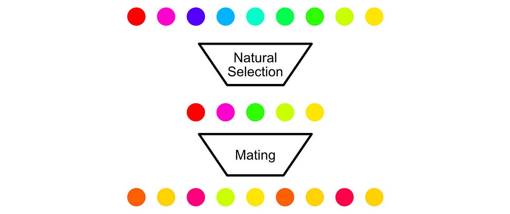
Evolution is the process of lifeforms changing over time as a result of “natural selection” influencing which characteristics are most common over successive generations.
Natural selection is the idea that only certain members of a population will live to the point of sexual maturity. If a member of a population has some disadvantageous trait they will be less likely to mate, and if a member of a population has some advantageous trait they will be more likely to mate.
In the short term, this can allow a species to adapt to shifting environments.

And in the long term, it can lead to the rise of new, highly optimized species.

Evolution relies on Deoxyribonucleic acid (DNA), a long and complex molecule that defines the genetic identity of an organism.
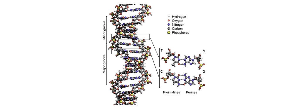
This structure can be simplified as a long series of genetic information. This genetic information influences things like eye color, height, proclivity to get certain diseases, etc.

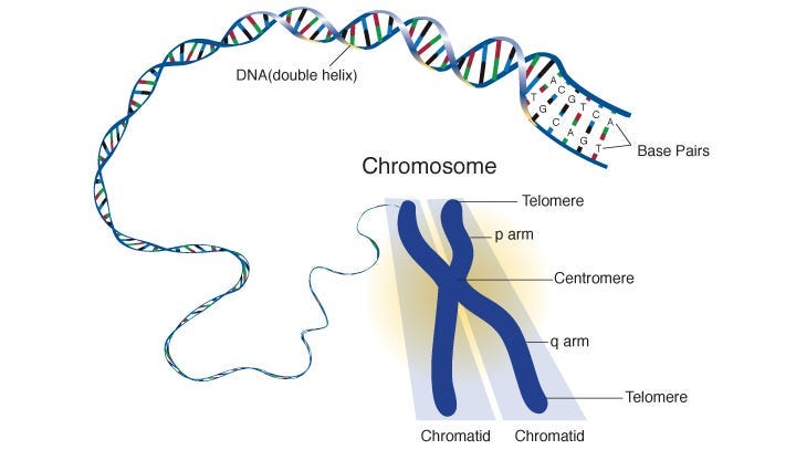
DNA is long and fragile, so for practical purposes it’s wrapped up into a structure called a chromosome.
During sexual reproduction, an offspring is created by dividing the chromosome of each parent at a random point, and swapping their genetic information. Thus, the offspring is a combination of both parent’s genetic information. This process is called “crossover”.

“Mutation” is another important concept in evolution, which involves the random modification of genetic information in a child offspring. Mutations can take a variety of forms: certain genetic information can be duplicated, removed, flipped around, etc.

Mutations can have no effect on an organism, can have a massive negative impact, or can occasionally introduce new traits in a species which are tremendously advantageous. The ability to see color, for instance, was the result of a single example of genetic material being produced four times.
the human eye uses four genes to make structures that sense light: three for cone cell or colour vision and one for rod cell or night vision; all four arose from a single ancestral gene. — Source
Most mutations cause no impact, or a negative impact. However, variation is vitally important for the species to maintain genetic diversity and evolve, so some mutation is critical for evolution to function.
That’s how evolution works in biology in a nutshell. Let’s explore how genetic algorithms manipulate these ideas to solve complex problems.
Genetic Algorithms
“Genetic Algorithms” (GAs) leverage the core principles of evolution to solve problems. The essential idea is to turn a problem into something resembling a chromosome, perform survival of the fittest, create breeding pairs and perform crossover, and then perform some random mutation to create a new population.
Let’s explore this through a practical example.
Imagine you were in charge of creating a schedule in a university. There are a bunch of rooms, classes, and teachers to teach them. Certain teachers may be capable of teaching only a handful of classes, certain classes need to be held in certain classrooms, etc. We can use a GA to help us solve this problem.
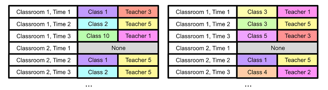
First, we can imagine the problem like DNA, where there’s a big list of locations and certain information that can exist in each of those locations. We can imagine each time slot in each classroom as a location, and the class and teacher as the information.

We can start off with a few randomly defined schedules, creating our initial “population”
Then, we can define something called a “fitness function”. We can look through our schedule and make some basic rules:
If a professor is teaching two classes at the same time, -20 fitness points
If a class is being held in a room that’s too small, -10 fitness points
etc.
We can apply this fitness function to our population, and preserve only the members of the population who are most fit.

Once we have a relatively fit population, we can randomly create breeding pairs and perform crossover on their information.

Then we can perform random mutation to inject some genetic diversity into the population.

If we do this, many many times, we’ll create successive generations which will slowly evolve to better fit our fitness function, thus giving us a good schedule!
Let’s code up this scheduling example and see how it works practically.
Have any questions about this article? Join the IAEE Discord.
Example 1) Scheduling
First, let’s define the problem we’re dealing with. Full code can be found here.
Imagine we have some collection of teachers, each of which is qualified to teach a certain set of subjects.
# teachers, and the subjects they can teach
teachers = {
    'Morgan': ['math', 'physics', 'statistics', 'computer science'],
    'Jordan': ['english', 'creative writing', 'drama', 'debate'],
    'Casey': ['biology', 'chemistry', 'psychology', 'sociology'],
    'Riley': ['history', 'geography', 'economics', 'business'],
    'Quinn': ['art', 'music', 'theater', 'french', 'german', 'spanish'],
    'Taylor': ['philosophy', 'ethics', 'english', 'health', 'physical education'],
    'Alex': ['robotics', 'engineering', 'environmental science']
}
Those teachers have to teach some number of classes, where each class has to be taught some number of times a week, may or may not need a computer lab, has a certain class size, etc.
classes = {
    'physics1': {'type': 'physics', 'weekly_instances': 3, 'requires_media': False, 'requires_computers': False, 'requires_chemlab': False, 'class_size': 20},
    'modern sculpture': {'type': 'art', 'weekly_instances': 2, 'requires_media': False, 'requires_computers': False, 'requires_chemlab': False, 'class_size': 15},
    'jazz': {'type': 'music', 'weekly_instances': 2, 'requires_media': True, 'requires_computers': False, 'requires_chemlab': False, 'class_size': 16},
    'calculus AB': {'type': 'math', 'weekly_instances': 3, 'requires_media': False, 'requires_computers': False, 'requires_chemlab': False, 'class_size': 18},
    'british literature': {'type': 'english', 'weekly_instances': 3, 'requires_media': False, 'requires_computers': False, 'requires_chemlab': False, 'class_size': 22},
    'french 1': {'type': 'french', 'weekly_instances': 2, 'requires_media': True, 'requires_computers': False, 'requires_chemlab': False, 'class_size': 17},
    'intro to psychology': {'type': 'psychology', 'weekly_instances': 2, 'requires_media': False, 'requires_computers': True, 'requires_chemlab': False, 'class_size': 20},
    'principles of sociology': {'type': 'sociology', 'weekly_instances': 2, 'requires_media': False, 'requires_computers': True, 'requires_chemlab': False, 'class_size': 19},
    'introduction to programming': {'type': 'computer science', 'weekly_instances': 3, 'requires_media': False, 'requires_computers': True, 'requires_chemlab': False, 'class_size': 20},
    'AP biology': {'type': 'biology', 'weekly_instances': 3, 'requires_media': False, 'requires_computers': False, 'requires_chemlab': True, 'class_size': 20},
    'chemistry fundamentals': {'type': 'chemistry', 'weekly_instances': 3, 'requires_media': False, 'requires_computers': False, 'requires_chemlab': True, 'class_size': 21},
    'debate and rhetoric': {'type': 'debate', 'weekly_instances': 2, 'requires_media': False, 'requires_computers': False, 'requires_chemlab': False, 'class_size': 18},
    'statistics and probability': {'type': 'statistics', 'weekly_instances': 3, 'requires_media': False, 'requires_computers': True, 'requires_chemlab': False, 'class_size': 23}
}
And each of those classes needs to be taught in a particular classroom:
rooms = {
    'Room 101': {'capacity': 30, 'has_media': False, 'has_computers': False, 'is_chemlab': False},
    'Room 102': {'capacity': 25, 'has_media': True, 'has_computers': False, 'is_chemlab': False},
    'Room 105': {'capacity': 30, 'has_media': True, 'has_computers': True, 'is_chemlab': False},
    'Art Studio A': {'capacity': 20, 'has_media': True, 'has_computers': False, 'is_chemlab': False},
    'Drama Stage': {'capacity': 25, 'has_media': True, 'has_computers': False, 'is_chemlab': False},
    'Gym A': {'capacity': 30, 'has_media': False, 'has_computers': False, 'is_chemlab': False},
    'Computer Lab 2': {'capacity': 20, 'has_media': False, 'has_computers': True, 'is_chemlab': False},
    'Chem Lab A': {'capacity': 20, 'has_media': False, 'has_computers': False, 'is_chemlab': True},
    'Lecture Hall 2': {'capacity': 35, 'has_media': True, 'has_computers': False, 'is_chemlab': False},
    'Language Lab': {'capacity': 20, 'has_media': True, 'has_computers': True, 'is_chemlab': False},
    'Philosophy Room': {'capacity': 18, 'has_media': False, 'has_computers': False, 'is_chemlab': False}
}
The goal is to come up with a good schedule, which is hard. If each room is available for 8 one hour time slots, 5 days a week, that’s 440 possible time slots in which one of 15 classes can be taught (including no class at all), and one of 8 teachers (including no teacher at all).
Doing some back-of-the-napkin math, that’s 120⁴⁴⁰ possible schedules. There are roughly 10⁸² atoms in the observable universe, meaning brute forcing this problem would be much harder than counting every atom in every known galaxy one at a time. Let’s solve this problem in a few minutes by making schedules have sex.
1.1) Defining the Population
First, we need to represent this problem in a way that’s similar to how DNA is structured. We can think of every possible time slot a room can have as a location in our DNA
"""Turning the problem into a structure that's similar to DNA
"""

import pandas as pd

# Parameters
num_periods = 8
num_days = 5

# Generate timeslots like "Period 1_Day 1", "Period 2_Day 3", etc.
timeslots = [f'Period {p+1}_Day {d+1}' for d in range(num_days) for p in range(num_periods)]

# Create list of room-timeslot pairs
data = [{'room': room, 'timeslot': timeslot} for room in rooms.keys() for timeslot in timeslots]

# Create DataFrame
df = pd.DataFrame(data)
df
We can then create random members of our population by simply filling in random classes and professors in each time slot.
"""Creating a random population member
"""

import random

def create_population_member():

    # Pull class names and teacher names
    class_names = list(classes.keys())
    teacher_names = list(teachers.keys())

    # Define probability of assigning None vs a valid entry
    none_prob = 0.2  # 20% chance of being None

    # Randomly assign class and teacher
    df['class'] = [random.choice(class_names + [None] * int(len(class_names) * none_prob)) for _ in range(len(df))]
    df['teacher'] = [random.choice(teacher_names + [None] * int(len(teacher_names) * none_prob)) for _ in range(len(df))]

    return df.copy(deep=True)

create_population_member()
Creating an initial population simply consists of calling this function numerous times, thus creating a set of random schedules.
population = [create_population_member() for _ in range(100)]1.2) Selection
Now that we have a random population, we need a way to calculate how “fit” a certain member of that population is. This can be done by simply iterating through all of the time slots and taking away points for things that are bad about the schedule.
"""Defining the fitness function. Here I'm calling the input
"chromosome", but it's simply a particular member of the population.

The result is a number, where 0 is a perfect fitness and imperfection
results in larger negative numbers.
"""

def fitness(chromosome):
    penalty = 0

    teacher_timeslot_set = set()
    class_instance_counter = {}

    for idx, row in chromosome.iterrows():
        class_name = row['class']
        teacher = row['teacher']
        room = row['room']
        timeslot = row['timeslot']

        if class_name is None or teacher is None:
            continue  # No assignment, skip

        # Track how many times this class is scheduled
        class_instance_counter[class_name] = class_instance_counter.get(class_name, 0) + 1

        # 1. Teacher qualified?
        class_info = classes[class_name]
        class_type = class_info['type']
        if class_type not in teachers.get(teacher, []):
            penalty += 10

        # 2. Room resources
        room_info = rooms[room]
        if class_info['requires_media'] and not room_info['has_media']:
            penalty += 5
        if class_info['requires_computers'] and not room_info['has_computers']:
            penalty += 5
        if class_info['requires_chemlab'] and not room_info['is_chemlab']:
            penalty += 5

        # 3. Room capacity
        if room_info['capacity'] < class_info['class_size']:
            penalty += (class_info['class_size'] - room_info['capacity'])

        # 4. Double-booked teacher
        key = (teacher, timeslot)
        if key in teacher_timeslot_set:
            penalty += 15
        else:
            teacher_timeslot_set.add(key)

    # 5. Penalize over/under-scheduling of classes
    for class_name, class_info in classes.items():
        required = class_info['weekly_instances']
        actual = class_instance_counter.get(class_name, 0)
        if actual != required:
            penalty += abs(required - actual) * 5  # Penalty per instance off

    return -penalty

fitness(population[0])
Here, I’m penalizing a schedule for the following:
if a teacher teaching a class is not qualified
if a class requires a certain type of resources that the room it’s in doesn’t have
if the room is smaller than the class size it holds
if a teacher is double-booked
if a class is being offered more or less often than it is supposed to be
The exact schedule we are optimizing for is directly defined in this fitness function, which is why GAs can be so powerful. By modifying these simple rules, we can change the nature of the schedule we get. If teachers complain about having too many classes without a break? Add a rule!
Once our fitness function has been defined, we can simply apply it to all of the members of our population (our random schedules) to preserve only the best ones.
"""Applying survival of the fittest
"""

def selection(population):
    # Evaluate fitness for each chromosome
    scored_population = [
        (chromosome, fitness(chromosome))
        for chromosome in population
    ]

    # Sort by fitness (higher is better)
    scored_population.sort(key=lambda x: x[1], reverse=True)

    # Keep top 50%
    num_survivors = len(population) // 2
    survivors = [chromosome for chromosome, _ in scored_population[:num_survivors]]

    return survivors

survivors = selection(population)
len(survivors)
1.3) Crossover
Now that half of their friends died, our schedules are probably feeling frisky. We can randomly create breeding pairs and have them perform crossover to create new offspring, bringing our population back to its original size.
"""performing crossover by randomly selecting a breeding pair
and creating an offspring. Here, crossover_rate dictates how much
swapping of information happens. 0.5 will result in an even division of
both parents, while larger or smaller numbers will bias parent 1 or 2.
"""

import random

def crossover(survivors, crossover_rate=0.5):
    original_population_size = len(survivors) * 2
    offspring = []

    while len(offspring) < len(survivors):
        # Pick two distinct parents
        parent1, parent2 = random.sample(survivors, 2)

        # Create a new child DataFrame
        child = parent1.copy()
        for idx in child.index:
            if random.random() < crossover_rate:
                child.at[idx, 'class'] = parent1.at[idx, 'class']
                child.at[idx, 'teacher'] = parent1.at[idx, 'teacher']
            else:
                child.at[idx, 'class'] = parent2.at[idx, 'class']
                child.at[idx, 'teacher'] = parent2.at[idx, 'teacher']

        offspring.append(child)

    return survivors + offspring

new_population = crossover(survivors)
len(new_population)
Here, we’re performing crossover by randomly swapping the class and teacher at a particular time slot of a particular room. The exact way crossover is done can be adjusted based on the application.
1.4) Mutation
Now that we’ve done crossover, we can mutate the population by injecting some random variance in the data. Just like crossover, the way you do this can depend on your application.
"""Randomly adjusting the classes and teacher for a given timeslot
to promote better results, I only choose a teacher that is qualified
to teach the new class.
"""
import random

def mutate(population, mutation_rate=0.01):
    class_names = list(classes.keys())

    for chromosome in population:
        for idx in chromosome.index:
            # Mutate class and teacher for a given classroom timeslot
            if random.random() < mutation_rate:
                new_class = random.choice(class_names + [None])
                chromosome.at[idx, 'class'] = new_class

                if new_class is None:
                    possible_teachers = list(teachers.keys()) + [None]
                else:
                    class_type = classes[new_class]['type']
                    possible_teachers = [
                        t for t, qualified_types in teachers.items()
                        if class_type in qualified_types
                    ] + [None]

                if possible_teachers:
                    chromosome.at[idx, 'teacher'] = random.choice(possible_teachers)

    return population


mutated_population = mutate(new_population)
len(mutated_population)
I chose to simply iterate through each time slot for every room and occasionally change both the class and the teacher teaching that class. Notice that None is a possible selection of both the teacher and the classroom. The way the fitness function is defined, if either the class or the teacher is None, then that particular timeslot for the room is treated as empty.
"""From the fitness function
"""
if class_name is None or teacher is None:
    continue  # No assignment, skip
So, this mutation function can add new classes and teachers to classroom timeslots, and can also make classroom time slots empty. The mutation_rate defines how likely it is for a particular time slot to be modified.
1.5) Tying it all together
So, we can create an initial population of random schedules, calculate their fitness, perform selection, crossover, and mutation. That’s everything that’s needed in a GA, so let’s hook it all up.
"""Optimizing schedules by creating an initial population
and iteratively performing selection, crossover, and mutation
"""
from tqdm import tqdm

# --- Set up GA loop ---
population_size = 40
generations = 300

#creating initial random population
population = [create_population_member() for _ in range(population_size)]

# for plotting, later
avg_fitness = []
min_fitness = []
max_fitness = []

for gen in tqdm(range(generations), desc="Evolving", dynamic_ncols=True):

    # calculating fitness of population
    scores = [fitness(chrom) for chrom in population]

    # keeping track of key data, for plotting
    avg = sum(scores) / len(scores)
    mn = min(scores)
    mx = max(scores)
    avg_fitness.append(avg)
    min_fitness.append(mn)
    max_fitness.append(mx)

    # making pretty output
    tqdm.write(f"Gen {gen} — avg: {avg:.1f}, min: {mn:.1f}, max: {mx:.1f}")

    # performing selection, crossover, and mutation to create a new population
    survivors = selection(population)
    population = crossover(survivors, crossover_rate=0.7)
    population = mutate(population, mutation_rate=0.005)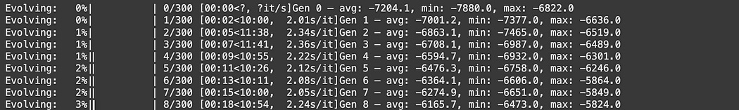
The initial population starts off performing poorly, which is expected because they’re completely random, but after a while, the population converges on near-perfect schedules.

If we plot out the history of fitness over time, we can see a consistent and steady improvement of the GA.
import matplotlib.pyplot as plt

# --- Plot results ---
plt.plot(avg_fitness, label='Average Fitness')
plt.plot(min_fitness, label='Min Fitness')
plt.plot(max_fitness, label='Max Fitness')
plt.xlabel('Generation')
plt.ylabel('Fitness')
plt.title('GA Fitness over Generations')
plt.legend()
plt.grid(True)
plt.show()
Recall that a fitness of 0 is a perfect schedule, so our GA did a pretty good job! You could take any schedule from the final population and it would be pretty solid. Of course, the “quality” of a schedule is defined by our fitness function. If we found that teachers were being forced to run back and forth across the school, we would want to make revisions to our fitness function.
You might notice that the fitness never quite reaches zero. That’s because, as a schedule becomes more perfect, it’s harder to find mutations that result in an improvement; most mutations harm the quality of a schedule in some way. If you let this run for a while you might find a good solution, or you could play around with the mutation rate and population size to perhaps converge on a perfect solution more quickly. GAs tend to run pretty quickly, so that type of experimentation is easy to do.
For now though, let’s explore how GAs can be applied in another type of problem.
Example 2) Traveling Salesman with Traffic
The “traveling salesman” is a famous problem in graph theory. The core idea is that you might have many cities connected to each other, and you need to figure out which route you should take to visit all cities in as little time as possible.
In this example, we’ll imagine that traffic patterns between the cities change over time. As our salesman is traveling from city to city, these traffic patterns will change. As we plan our route between cities, we ought to account for those traffic patterns.
I’m sure there’s some clever way to optimize for this, but I don’t know it. One of the cool things about genetic algorithms is how easy they are to apply to problems, so let’s just throw a GA at it and see what happens!
Example 2.1) Defining the problem
First, we need to define the data we’re playing with. The whole idea is that there’s a route between each city and the time it takes to traverse from one city to another changes over time. I’m actually storing that information as a directed graph, where each edge has a list of traversal times for every hour in the day. We can get the graph of traversal times at a particular time of day by sampling this graph.
"""Defining a graph with changing traffic patterns over time.
"""

import random
import networkx as nx
import matplotlib.pyplot as plt

def generate_time_dependent_graph(cities):
    graph = {}
    for from_city in cities:
        graph[from_city] = {}
        for to_city in cities:
            if from_city != to_city:
                graph[from_city][to_city] = [random.randint(1, 4) for _ in range(24)]
    return graph

def get_graph_at_hour(graph, hour):
    hourly_graph = nx.DiGraph()
    for from_node, edges in graph.items():
        for to_node, weights in edges.items():
            hourly_graph.add_edge(from_node, to_node, weight=weights[hour])
    return hourly_graph

def draw_graphs_for_hours(graph, hours):
    fig, axes = plt.subplots(1, len(hours), figsize=(16, 4))
    pos = nx.spring_layout(nx.DiGraph(graph))  # fixed layout for all graphs

    for idx, hour in enumerate(hours):
        G_hour = get_graph_at_hour(graph, hour)
        ax = axes[idx]
        ax.set_title(f'Hour {hour}')
        nx.draw(G_hour, pos, ax=ax, with_labels=True, node_color='lightblue', node_size=800, arrows=True)
        labels = nx.get_edge_attributes(G_hour, 'weight')
        nx.draw_networkx_edge_labels(G_hour, pos, edge_labels=labels, ax=ax, font_size=8)

    plt.tight_layout()
    plt.show()

# Create the graph and visualize it
cities = ['A', 'B', 'C', 'D', 'E', 'F', 'G', 'H', 'I', 'J', 'K', 'L', 'M']
time_dependent_graph = generate_time_dependent_graph(cities)

# Render for 4 sample hours
draw_graphs_for_hours(time_dependent_graph, hours=[0, 6, 12, 18])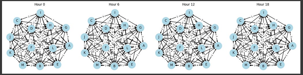
If this looks like french to you, check out my article on graphs:

And, that’s really the most difficult part. Defining a GA to solve this problem is virtually identical to the previous example we discussed.
Example 2.2) Defining the GA
Just like in the previous example, we’ll need to format the structure into something resembling DNA, define a fitness function, do selection, crossover, and then mutation.
Defining the DNA is pretty straightforward, it can just be a list of cities in some order. Here I’m calling it a genome rather than DNA, the analogies between GAs and their biological inspiration can get a bit handwavy.
"""Defining initial population
"""

genome_length = 2 * len(cities)
population = [
    [random.choice(cities) for _ in range(genome_length)]
    for _ in range(pop_size)
]
Here, I decided to make the genome long because, in theory, it might be optimal to travel through a city than to drive directly from one city to another. I wanted to allow for some room in a population member to have long lists and be able to explore those types of solutions.
The fitness function, evaluate_genome takes a particular genome (aka population member, aka DNA, aka solution… Whatever). and assigns a fitness score to it.
def evaluate_genome(genome, graph_data, start_city):
    current_time = 0
    current_city = start_city
    visited = set([current_city])

    for next_city in genome:
        if next_city == current_city:
            continue

        graph_at_time = get_graph_at_hour(graph_data, current_time % 24)
        if not graph_at_time.has_edge(current_city, next_city):
            continue

        travel_time = graph_at_time[current_city][next_city]['weight']
        current_time += travel_time
        current_city = next_city
        visited.add(current_city)

        if len(visited) == len(graph_data):
            break

    return -current_time if len(visited) == len(graph_data) else -float('inf')
Here, the fitness is -infinity if a city in the list was missed. The idea is that we want to go to all cities, so a genome is bad if it doesn’t cover every city.
If all the cities were traveled to, the fitness is the negative of the time that took. Thus, faster routes result in a better reward. Here, the fitness function essentially runs a simulation of moving from city to city. It gets the graph of the current traffic patterns at a particular period of time, adds the traversal time for the current move, etc.
I also have a random crossover and mutation function, just like before.
def mutate(genome, cities, mutation_rate=0.1):
    new_genome = genome[:]
    for i in range(len(new_genome)):
        if random.random() < mutation_rate:
            new_genome[i] = random.choice(cities)
    return new_genome

def crossover(parent1, parent2):
    return [random.choice([g1, g2]) for g1, g2 in zip(parent1, parent2)]
And I wrap that all up with some helper functions and send it.
import random

def evaluate_genome(genome, graph_data, start_city):
    current_time = 0
    current_city = start_city
    visited = set([current_city])

    for next_city in genome:
        if next_city == current_city:
            continue

        graph_at_time = get_graph_at_hour(graph_data, current_time % 24)
        if not graph_at_time.has_edge(current_city, next_city):
            continue

        travel_time = graph_at_time[current_city][next_city]['weight']
        current_time += travel_time
        current_city = next_city
        visited.add(current_city)

        if len(visited) == len(graph_data):
            break

    return -current_time if len(visited) == len(graph_data) else -float('inf')

def mutate(genome, cities, mutation_rate=0.1):
    new_genome = genome[:]
    for i in range(len(new_genome)):
        if random.random() < mutation_rate:
            new_genome[i] = random.choice(cities)
    return new_genome

def crossover(parent1, parent2):
    return [random.choice([g1, g2]) for g1, g2 in zip(parent1, parent2)]

def run_generation(population, graph, cities, start_city, mutation_rate=0.1):
    scored_population = [(genome, evaluate_genome(genome, graph, start_city)) for genome in population]
    scored_population.sort(key=lambda x: x[1], reverse=True)

    next_generation = [genome for genome, _ in scored_population[:2]]  # elitism

    while len(next_generation) < len(population):
        parent1, parent2 = random.choices(scored_population[:5], k=2)
        child = crossover(parent1[0], parent2[0])
        mutated_child = mutate(child, cities, mutation_rate)
        next_generation.append(mutated_child)

    return next_generation, scored_population[0]

def genetic_algorithm(graph, cities, start_city='A', generations=10, pop_size=500, mutation_rate=0.1):
    genome_length = 2 * len(cities)
    population = [
        [random.choice(cities) for _ in range(genome_length)]
        for _ in range(pop_size)
    ]

    best_overall = (None, -float('inf'))
    for gen in range(generations):
        population, best = run_generation(population, graph, cities, start_city, mutation_rate)
        if best[1] > best_overall[1]:
            best_overall = best
        print(f"Generation {gen+1}: Best fitness = {best[1]}")

    print("\nBest path found:", best_overall[0])
    print("Final fitness:", best_overall[1])
    return best_overall

# --- Run the GA on your existing graph ---
best_path, best_fitness = genetic_algorithm(time_dependent_graph, cities)
Notice that there are some repeated characters in the best solution found. Because of the way we define our fitness function, these are simply skipped. Also, we stop counting once all the cities have been accessed. So, the real result is:
L, F, D, K, B, M, C, E, J, G, I, H, F, K, J, AWhere each letter represents a city. That’s 21 hours to go through all 16 cities. One drawback of GAs is that, often, we have no idea if the solution we end up with is optimal. That said, if you’re working in a use case where “good enough” is good enough, then GAs are a fantastic choice. Considering the average time to traverse from one city to another is two hours, that result is much better than average!
Conclusion
In this article we watched schedules have sex like a bunch of creeps.
Haven’t you people ever heard of, closing the god damn door, no?
Jokes aside, we actually learned about a very powerful approach to solving arbitrary problems. If you can turn your problem into a representation that is similar to DNA, and define a fitness function that makes some amount of sense, you can use genetic algorithms to quickly find compelling solutions!