
Positional Encoding — Intuitively and Exhaustively Explained
How modern AI understands space and time


In this article we’ll form a thorough understanding of positional encoding, a fundamental tool that allows AI models to understand ideas of space and time.
We’ll start by exploring the transformer (the grandfather of today's modern AI models) and why it needs additional positional information to be provided along with the input. We’ll then work through increasingly sophisticated methods of introducing positional information to transformer style models to build a thorough conceptual understanding of the approach.
By the end of this article you’ll understand why positional encoding plays a fundamental role in the performance of modern AI systems, and several approaches to do positional encoding.
Who is this useful for? Anyone interested in forming a deep understanding of modern AI.
How advanced is this post? This article contains intuitive descriptions of complex ideas, and is thus relevant to readers of all levels. Some of the sections have implementation that may be relevant to more advanced readers.
Prerequisites: I’ll do my best to provide all foundational information so that you can forge a thorough conceptual understanding without prior AI experience. That said, this is a fairly nuanced topic. I’ll have references to supplementary information throughout the article should you find yourself lost.
The Transformer, How LLMs Work, and Why They Need Positional Information
Before we get into the various forms of positional encoding, let’s first discuss why LLMs need positional encoding in the first place. Imagine you feed in the following sequence to an LLM:
Joe is six foot. Bob is five seven. Who is taller?The relative position of certain words is important. Imagine if we shuffled some of the words around:
Bob is six foot. Joe is five seven. taller who is?The meaning completely changes. Even worse, if you really shuffle the words around, all meaning is completely lost
Joe taller? foot. is Bob Who is is seven. five sixThus, for any LLM to do pretty much anything with text, it has to have some understanding of the order of the input sequence.
To the uninitiated this might appear to be a simple problem. If you want the sequence to be in order, you just pass the sequence to your AI model in order. In fact, with many forms of AI models this is sufficient; many older and simpler AI strategies like recurrent neural networks, convolutional networks, and classic neural networks have a strong ability to understand the order of an input implicitly.
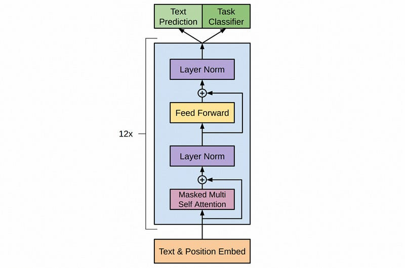
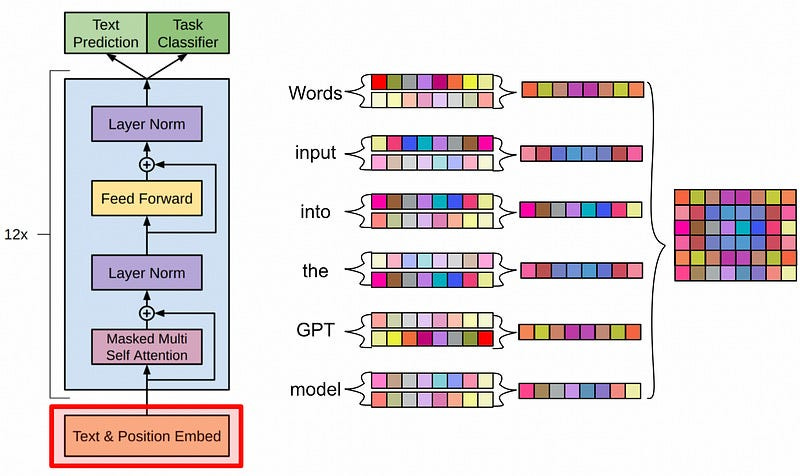
Modern LLMs don’t use these older strategies. Instead, they use a fairly new modeling architecture called the “transformer”. Transformers allow any word to interact with any other word, instead of only allowing nearby information to interact.

This arbitrary interaction allows the model to create a robust understanding of the entire input, but the added complexity makes it very hard for the model to implicitly understand the order of the input. To hammer home this idea, I’d like to take a moment to explore how a model like GPT works.
How Data Flows Through a Transformer, and Why That Breaks Position
Let’s imagine we have some LLM, like GPT.
Then imagine we pass GPT the following query
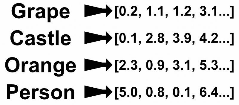
Translate to French: I am a managerOur input is first passed through a text embedding. This turns our sequence of words into a sequence of vectors. By turning words into vectors, we allow the LLM to reason mathematically about how words relate with other words.
Our input is also treated with a positional encoding, which we’ll talk about in a bit. For now, we’ll skip this step to explore why positional encoding is necessary.

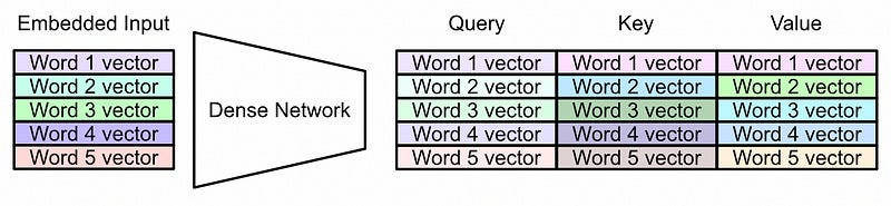
Now that we have a vector that’s associated with each word, we can pass that through a system called “self-attention”. In self attention we first use a neural network to convert our input representation into three different representations.
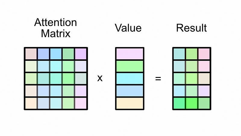
Then, the representation called the query and key are multiplied together and used to create something called an “attention matrix”

This attention matrix is then multiplied by the value matrix, resulting in the output of self-attention
There’s a bunch of math we would need to cover to thoroughly understand this mechanism. It’s not incredibly complicated, I have several articles on the subject that will allow you to completely understand it if you’re interested:


But, for our purposes, there’s one critical concept I’d like to discuss.
When you multiply the attention matrix by the value matrix, each row in the attention matrix essentially functions as a set of weights dictating how rows should be combined to create the output.
Here’s an example of multiplying an attention matrix by a value matrix from the “Multi-Headed Self Attention — By Hand” article:
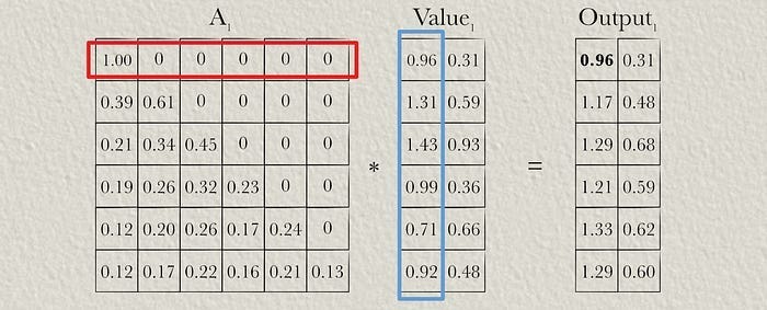
The first row in the output is equivalent to the first row in the value matrix because the first row in attention is 100% the first value, and 0% all of the other values. If we move onto the next row in the output, it’s a combination of 39% of the first row and 61% of the second row in the value matrix, as specified by the attention matrix.
Recall that we calculated the attention matrix by multiplying the query and key together.
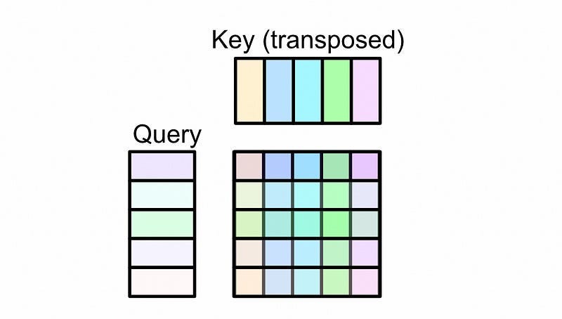
Because of the way matrix multiplication works, the values in the attention matrix are not governed at all by the location of a word in a sequence. Rather, they’re solely governed by the values of the word vectors in the query and key. If the query and key multiplied together to create an attention matrix that looked something like this:
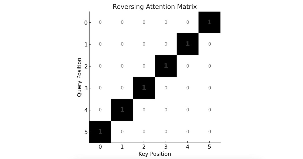
Then multiplying this matrix by the value matrix would produce a perfectly reversed output.
So, in allowing word vectors to arbitrarily interact with one another (one of the fundamental strengths of the transformer), the transformer has the ability to destroy all sense of order within the sequence. The thing that governs the order of the sequence, the attention matrix, is calculated by the values of the word vectors, not their location. Thus, LLMs can very easily destroy all sense of position within an input. Let’s explore how the original transformer got around this problem.
Additive Sinusoidal Positional Encoding
The creators of the original transformer architecture were confronted with the issue of their new model losing the order of inputs, and had to find a way to solve it. They elected to do that with a strategy commonly referred to as “additive sinusoidal positional encoding”
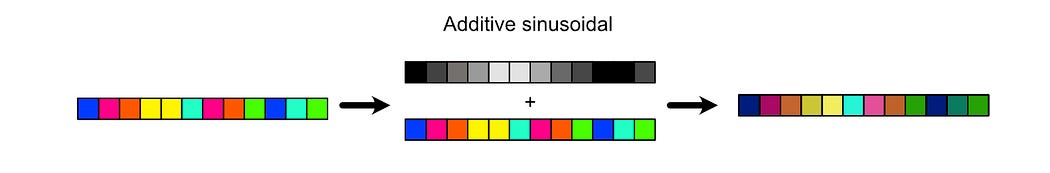
Essentially, the idea is to bake positional information into the values of the vectors that represent each word. Recall that one of the first steps of feeding words into a transformer style model is to convert those words into vectors.
In the original transformer paper, they essentially generated wiggly lines for each spot in the input, where the lines got progressively more wiggly throughout locations in the input sequence. They added these wiggly lines to the word vectors, constructing vectors that represent both the values of words as well as their locations in the input sequence.
Now, because each vector has positional information, the model can use that information when constructing queries and keys,

which in turn dictate the creation of the attention matrix

Which, ultimately, dictates how words are contextualized together.

In this strategy, positional information is added to the word vectors that are input into the model. It’s then the models job to learn parameters which reason about that information effectively. Let’s get an idea of how this might work with a toy problem.
Exploring Additive Sinusoidal Positional Encoding With a Toy Problem
Imagine the following problem:
Given a sequence of random numbers, can we make a transformer style model
that can tell us the index of the largest number in the sequence?
Naturally, this requires a model to understand position, as the task requires the model to return the location of the largest value in the input sequence. Let’s try implementing a transformer style model with additive sinusoidal positional encoding, and see if it’s up to the job. Full code can be found here.
First, we’ll create a function that defines our modeling objective. This simply returns a list of random numbers, and the corresponding maximum index.
# --- Data: Predict index of max token ---
def generate_batch(num, seq_len):
    x = torch.randint(1, vocab_size, (num, seq_len))
    y = torch.argmax(x, dim=1)
    return x.to(device), y.to(device)
Notice how we generate numbers between one and vocab_size. Transformers require us to create a vector for each word in our vocabulary. Here, each word is a number between 1 and whatever vocab_size is specified to be, in this case 20. seq_len defines how long the sequence we generate will be.
Before we implement the transformer, let’s implement the positional encoding which the transformer will use.
# --- Sinusoidal Positional Encoding ---
def sinusoidal_encoding(seq_len, d_model, device):
    position = torch.arange(seq_len, dtype=torch.float, device=device).unsqueeze(1)
    div_term = torch.exp(torch.arange(0, d_model, 2, device=device) * (-math.log(10000.0) / d_model))
    pe = torch.zeros(seq_len, d_model, device=device)
    pe[:, 0::2] = torch.sin(position * div_term)
    pe[:, 1::2] = torch.cos(position * div_term)
    return pe  # [seq_len, d_model]
this function accepts seq_len, which is important because we need that to know how many squiggly lines we need to make. d_model, on the other hand, defines how long those squiggly lines need to be. That will be whatever length we use to represent the words (or, in this case, numbers) in our vocabulary. Having a squiggly line for each spot in the sequence, and having those squiggly lines represented as vectors that are the same length as the word vectors, will make applying the positional encoding as easy as adding the two vectors together.

To facilitate actually creating our positional encoding, we first generate a list of indexes with position = torch.arange(seq_len, dtype=torch.float, device=device).unsqueeze(1). This gets us an array of positions like.
[0, 1, 2, ..., seq_len-1]The rest is excessively complicated given how conceptually simple the approach is, and I don’t want to waste a bunch of time unpacking all of the math. The positional encoding formula for this approach looks like this:

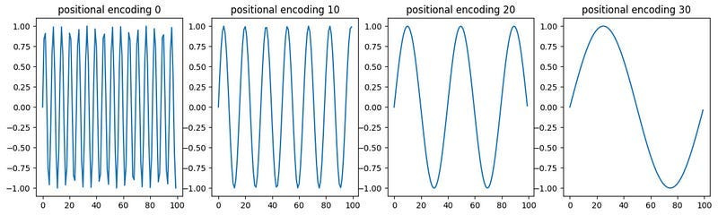
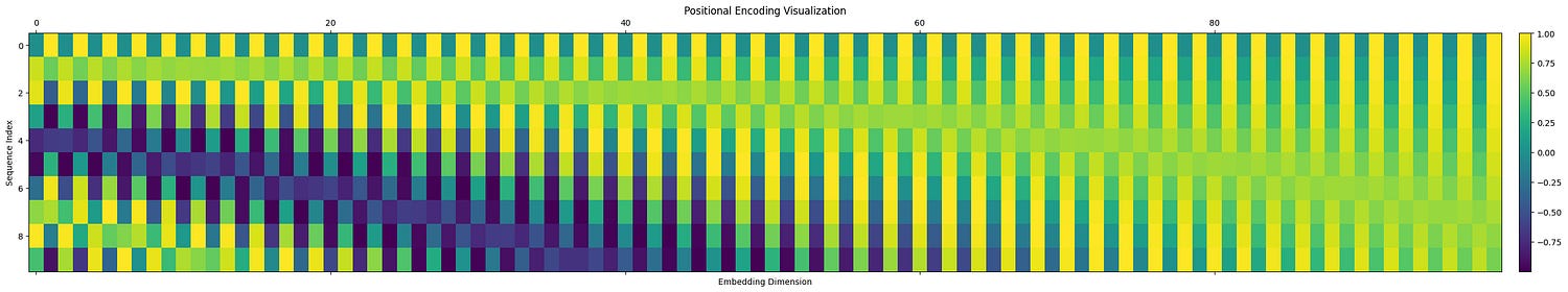
Which, if you’re familiar with trigonometry, you might realize that these are sin and cosine functions. Here, pos represents the location of a particular word within the sequence, and we’re modifying the frequency both by i, the location in the embedding vector, and dmodel, the size of the model. The final positional encoding vectors look something like this:
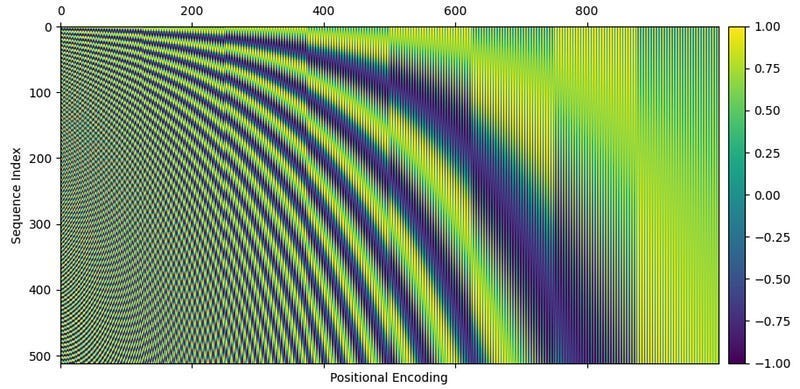
In the image above, each row represents the squiggly line that would be added to a word. with subsequent rows representing subsequent words. Here’s the same plot, but with a smaller model dimension and smaller sequence length to aid in visibility.
We can use our generated positional encodings within a transformer, like so:
# --- Config ---
device = "cuda" if torch.cuda.is_available() else "cpu"
vocab_size = 20
d_model = 16
n_heads = 4
train_seq_len = 64
num_train = 30000
num_test = 500
batch_size = 64
epochs = 10
num_layers = 2

# --- Transformer Model ---
class MaxIndexTransformer(nn.Module):
    def __init__(self, seq_len, num_layers):
        super().__init__()
        self.token_emb = nn.Embedding(vocab_size, d_model)
        self.pos_enc = sinusoidal_encoding(seq_len, d_model, device)
        self.layers = nn.ModuleList([
            nn.TransformerEncoderLayer(d_model=d_model, nhead=n_heads, batch_first=True)
            for _ in range(num_layers)
        ])
        self.norm = nn.LayerNorm(d_model)
        self.classifier = nn.Linear(d_model, 1)

    def forward(self, x):
        tok = self.token_emb(x)
        pos = self.pos_enc[:x.size(1)]
        tok = tok + pos
        for layer in self.layers:
            tok = layer(tok)
        logits = self.classifier(tok).squeeze(-1)  # [B, T]
        return logits
Here we’re defining a transformer style model with PyTorch. It has a word embedding for each word as defined by
self.token_emb = nn.Embedding(vocab_size, d_model)and we also pre-calculate positional embeddings
self.pos_enc = sinusoidal_encoding(seq_len, d_model, device)When we go to make an inference with the model, we add the positional information to the embeddings with
tok = tok + posbefore passing the tokens through the model.
Recall that our toy problem was to find the index of the largest value in the sequence. We can train and evaluate our model on a few examples and see that the model can performantly identify the largest value in the input sequence.
# --- Train ---
def train(model, optimizer, criterion):
    model.train()
    for _ in range(epochs):
        for _ in range(num_train // batch_size):
            x, y = generate_batch(batch_size, train_seq_len)
            logits = model(x)
            loss = criterion(logits, y)
            optimizer.zero_grad()
            loss.backward()
            optimizer.step()

# --- Evaluate ---
@torch.no_grad()
def evaluate(model, seq_len):
    model.eval()
    x, y = generate_batch(num_test, seq_len)
    logits = model(x)
    preds = torch.argmax(logits, dim=1)
    acc = (preds == y).float().mean().item()
    print(f"Eval acc at seq_len={seq_len}: {acc:.3f}")
    return acc

# --- Run ---
model = MaxIndexTransformer(seq_len=train_seq_len, num_layers=num_layers).to(device)
optimizer = torch.optim.Adam(model.parameters(), lr=1e-3)
criterion = nn.CrossEntropyLoss()

train(model, optimizer, criterion)
evaluate(model, train_seq_len)
Thus, we’ve seen how the addition of additive sinusoidal positional encoding can impart a transformer style model with the ability to understand sequence order.
Learned Positional Encodings
OpenAI famously took ideas from the transformer and built on them with GPT. One of the many things they changed was how GPT handled positional encoding.
Instead of using some fancy math to create fancy squiggly lines for each location in a sequence, GPT simply created a vector for each spot in the sequence and had the model learn what values make sense in each spot.

Actually implementing this is super straightforward. Instead of doing a bunch of fancy math to make squiggly lines, we just use nn.Embedding to create a vector for each spot in our sequence (called pos_emb)
# --- Transformer with Learned Positional Embedding ---
class MaxIndexTransformer(nn.Module):
    def __init__(self, seq_len, num_layers):
        super().__init__()
        self.token_emb = nn.Embedding(vocab_size, d_model)
        self.pos_emb = nn.Embedding(seq_len, d_model)
        self.layers = nn.ModuleList([
            nn.TransformerEncoderLayer(d_model=d_model, nhead=n_heads, batch_first=True)
            for _ in range(num_layers)
        ])
        self.norm = nn.LayerNorm(d_model)
        self.classifier = nn.Linear(d_model, 1)

    def forward(self, x):
        batch_size, seq_len = x.size()
        positions = torch.arange(seq_len, device=x.device).unsqueeze(0).expand(batch_size, seq_len)
        tok = self.token_emb(x) + self.pos_emb(positions)
        for layer in self.layers:
            tok = layer(tok)
        logits = self.classifier(tok).squeeze(-1)  # [B, T]
        return logits
When we go to make an inference, we simply add the word and position embedding together with
tok = self.token_emb(x) + self.pos_emb(positions)Running this model on our toy problem (finding the max index in a random sequence), we get almost 100% accuracy. I’m just playing around, and could almost certainly modify this training code to be 100% accurate, so this is functionally identical to the 100% accuracy we saw in sinusoidal positional encoding.

The authors of the original GPT paper claimed that learned positional encoding resulted in superior output to additive sinusoidal approaches. It’s also super easy to implement it, which is why I used this approach when creating a transformer style model designed to solve a rubik’s cube.
Relative Positional Encoding
Both of the encoding strategies we’ve discussed previously are examples of “absolute” positional encoding, meaning the information added to the word vectors denotes the actual location of the vector in the sequence. One problem with this approach is that sequences that are longer than the model saw during training can significantly degrade the performance of the model, as the model has never seen information about those locations in the training set.

The paper Transformer-XL: Attentive Language Models Beyond a Fixed-Length Context built on top of previous positional encoding strategies with a single objective: making transformer style models that can understand sequences than are larger than the ones they were trained on.
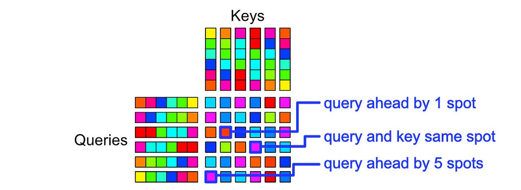
One of the central ideas of transformer XL was to use relative positional encoding. Instead of tokens being enumerated based on how far they were to the beginning of the sequence, like in previous approaches:
token 0, token 1, token 2, token 3, .... token nThey, instead, enumerated the tokens based on how far they were to the last token.
token n ... token 3, token 2, token 1, token 0This is incredibly powerful because, as a model generates new tokens, the most recently generated tokens in the sequence are the most important. If I gave an LLM the following phrase, for instance:
I don't know about you, but I think an elephant would
easily crush a can if it stepped on it. Elephants are
very _______
The information at the end of the sequence is more relevant than the information at the beginning of the sequence when filling in the blank. If a model is especially good at understanding information at the end of the sequence, it will be better at generating output, even if the sequence becomes very large.
One practical issue with this approach is that, as you generate a sequence, the positional information for each token has to change. The first token generated is at position zero, then when another token is generated it’s kicked over to spot one, then two, etc.
0
1, 0
2, 1, 0
3, 2, 1, 0
...
Both of the previous approaches injected positional information about each word at the beginning of the model.

Then, these vectors (with their positional information) are passed through a big (and expensive to run) LLM. To re-calculate new values with new positional information, you would have to change the positional information at the input and recalculate all of the inputs throughout the entire model. For every token generated. That would be ludicrously expensive.
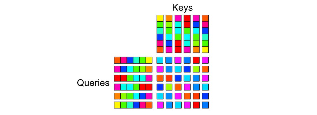
To deal with this problem, the authors of the Transformer XL paper shifted where positional information is injected. Instead of injecting positional information at the input, then calculating how word vectors should attend to one another
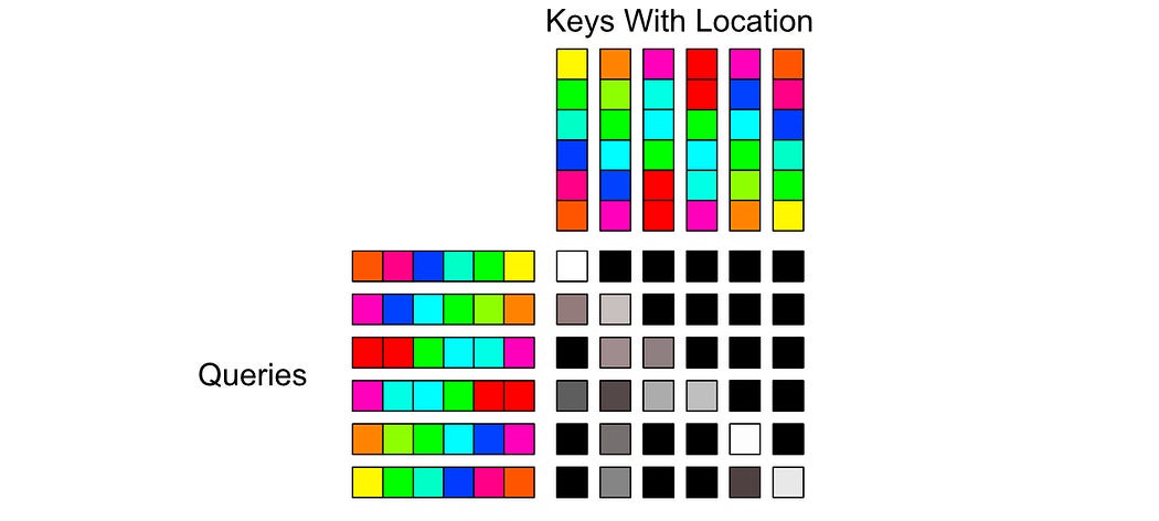
They calculate scores based on content and position separately
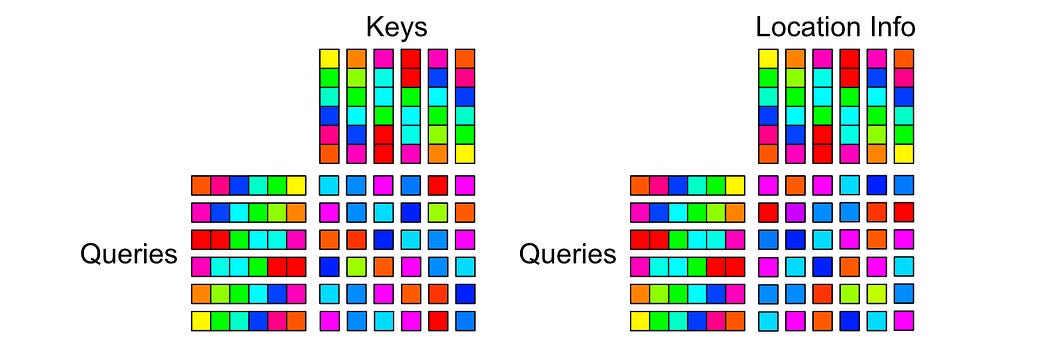
And combine them together to calculate how tokens should attend with one another.
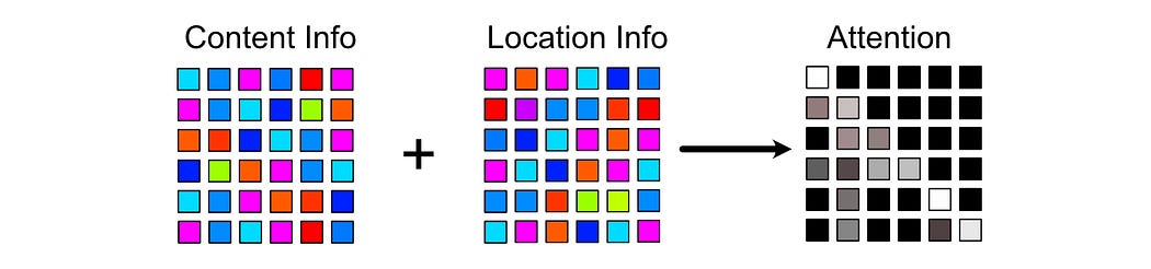
This allowed the authors of the Transformer XL paper to modify positional information after a token was already generated, meaning you can maintain relative positional information without needing to recalculate every token at every generated step.
It’s worth noting, the actual positional information could be learned, or it could be sinusoidal. The authors of the transformer XL paper favored sinusoidal encoding like the original transformer, as continuous functions allow the model to extrapolate it’s understanding of position further into the past.
I’ll probably cover Transformer XL, and similar approaches like DeBERTa, in isolation in other articles. The general approach is fascinating, but there’s a lot of subtlety in the approach and how it relates with sequence modeling, which is deserving of it’s own article. For now, I think it’s sufficient to understand the major contribution of Transformer XL: it encodes positional information relative to the most recent token instead of relative to the first token, and it does that by cleverly injecting positional information within the attention mechanism itself, rather than at the input of the model. We’ll discuss strategies that take this general idea and run with it.
Bucket Relative Bias
Because the Transformer XL paper has the goal of working with arbitrarily large sequences, the authors of the Transformer XL paper invest a lot of computational resources into modeling position. This results in a model which is very expressive about positional information, but at the cost of complexity.
The authors of the T5 paper did not have this objective (The T5 paper is a metastudy about transfer learning, without an explicit focus on studying positional embedding). Thus, the T5 paper uses a positional encoding scheme which is inspired by the Transformer XL paper, but simplifies the approach significantly. There are two key deviations the T5 paper made from the original Transformer XL approach:
They represent positional information as a learned bias that gets added to attention
They group certain distances between queries and keys into buckets
This allowed the T5 paper to very efficiently model relative position. To make it happen, you calculate attention scores like normal:
calculate how far apart those two tokens are
grab the bias term corresponding to the bucket containing each distance

add the relevant biases to the attention scores, then softmax to calculate attention.
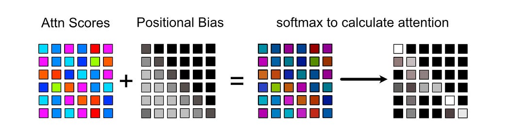
The only real subtlety is the way buckets are defined. The T5 Paper defines:
a set of buckets for small, exact differences for keys that are before the query in the sequence
a set of buckets for small, exact differences for keys that are after the query in the sequence
a set of buckets for large, inpercise differences for keys that are before the query in the sequence
a set of buckets for large, inpercise differences for keys that are after the query in the sequence
Here’s an implementation of a PyTorch module with learnable biases corresponding to where relative positions fall into certain buckets.
# --- T5 Relative Positional Bias ---
class T5RelativePositionalBias(nn.Module):
    def __init__(self, n_heads, num_buckets=32, max_distance=128):
        super().__init__()
        self.n_heads = n_heads
        self.num_buckets = num_buckets
        self.max_distance = max_distance
        self.relative_attention_bias = nn.Embedding(num_buckets, n_heads)

    def _relative_position_bucket(self, relative_position):
        num_buckets = self.num_buckets
        max_distance = self.max_distance

        # Bidirectional bucketing
        num_buckets //= 2
        relative_buckets = (relative_position > 0).to(torch.long) * num_buckets
        relative_position = torch.abs(relative_position)

        # Small positions map directly to buckets
        max_exact = num_buckets // 2
        is_small = relative_position < max_exact

        # Large positions get log-scaled buckets
        relative_position_if_large = max_exact + (
            torch.log(relative_position.float() / max_exact) /
            math.log(max_distance / max_exact) * (num_buckets - max_exact)
        ).to(torch.long)
        relative_position_if_large = torch.min(
            relative_position_if_large,
            torch.full_like(relative_position, num_buckets - 1)
        )

        # Combine buckets
        relative_buckets += torch.where(is_small, relative_position, relative_position_if_large)
        return relative_buckets

    def forward(self, seq_len):
        q_pos = torch.arange(seq_len, dtype=torch.long, device=self.relative_attention_bias.weight.device)
        rel_pos = q_pos[:, None] - q_pos[None, :]
        buckets = self._relative_position_bucket(rel_pos)
        bias = self.relative_attention_bias(buckets)  # [T, T, H]
        return bias.permute(2, 0, 1).unsqueeze(0)    # [1, H, T, T]
We can then define a layer of a transformer style model that uses these relative attention biases like so:
# --- T5 Transformer Layer ---
class T5TransformerEncoderLayer(nn.Module):
    def __init__(self, d_model, n_heads, dropout=0.1):
        super().__init__()
        self.norm1 = nn.LayerNorm(d_model)
        self.norm2 = nn.LayerNorm(d_model)

        # Attention projections
        self.q_proj = nn.Linear(d_model, d_model)
        self.k_proj = nn.Linear(d_model, d_model)
        self.v_proj = nn.Linear(d_model, d_model)
        self.out_proj = nn.Linear(d_model, d_model)

        self.head_dim = d_model // n_heads

    def forward(self, x, relative_attention_bias):
        # Pre-LayerNorm attention
        residual = x
        x_norm = self.norm1(x)

        # Project to query/key/value
        B, T, _ = x_norm.shape
        q = self.q_proj(x_norm).view(B, T, n_heads, self.head_dim).transpose(1, 2)
        k = self.k_proj(x_norm).view(B, T, n_heads, self.head_dim).transpose(1, 2)
        v = self.v_proj(x_norm).view(B, T, n_heads, self.head_dim).transpose(1, 2)

        # Attention scores
        attn_scores = torch.matmul(q, k.transpose(-2, -1)) / math.sqrt(self.head_dim)
        attn_scores = attn_scores + relative_attention_bias

        # Attention weights
        attn_weights = F.softmax(attn_scores, dim=-1)

        # Context
        context = torch.matmul(attn_weights, v)
        context = context.transpose(1, 2).contiguous().view(B, T, -1)
        context = self.out_proj(context)

        # Residual connection
        x = residual + context

        # Final LayerNorm (no FFN)
        x = x + self.norm2(x)
        return x
This is a minimal implementation of an encoder block. Usually you’d also have a feed forward network in here as well, but we’re keeping it simple in this example.
You might notice that relative_attention_bias is accepted as an input to the forward function. If you wanted each layer of the model to learn it’s own positional parameters, you could define a seperate learnable T5RelativePositionalBias for each layer, but the authors of the T5 paper elected for all layers in the model to share the same bias information. As a result, the biases are passed to the encoder block, rather than stored within the block directly.
As we previously discussed, these biases are added to the attention scores calculated by the multiplication of the query and key, and those biased attention scores are then softmaxed to calculate attention.
We can then build a model that uses these relatie biases and encoder blocks.
# --- Transformer Model ---
class MaxIndexTransformer(nn.Module):
    def __init__(self, seq_len, num_layers):
        super().__init__()
        self.token_emb = nn.Embedding(vocab_size, d_model)
        self.relative_bias = T5RelativePositionalBias(n_heads)
        self.layers = nn.ModuleList([
            T5TransformerEncoderLayer(d_model, n_heads)
            for _ in range(num_layers)
        ])
        self.norm = nn.LayerNorm(d_model)
        self.classifier = nn.Linear(d_model, 1)

    def forward(self, x):
        tok = self.token_emb(x)
        T = x.size(1)
        rel_bias = self.relative_bias(T)

        for layer in self.layers:
            tok = layer(tok, rel_bias)

        tok = self.norm(tok)
        logits = self.classifier(tok).squeeze(-1)
        return logits
We can then train this model on our task of finding the index of the largest value in the sequence.
# --- Train ---
def train(model, optimizer, criterion):
    model.train()
    for _ in range(epochs):
        for _ in range(num_train // batch_size):
            x, y = generate_batch(batch_size, train_seq_len)
            logits = model(x)
            loss = criterion(logits, y)
            optimizer.zero_grad()
            loss.backward()
            optimizer.step()

# --- Evaluate ---
@torch.no_grad()
def evaluate(model, seq_len):
    model.eval()
    x, y = generate_batch(num_test, seq_len)
    logits = model(x)
    preds = torch.argmax(logits, dim=1)
    acc = (preds == y).float().mean().item()
    print(f"Eval acc at seq_len={seq_len}: {acc:.3f}")
    return acc

# --- Run ---
model = MaxIndexTransformer(seq_len=train_seq_len, num_layers=num_layers).to(device)
optimizer = torch.optim.Adam(model.parameters(), lr=1e-3)
criterion = nn.CrossEntropyLoss()

train(model, optimizer, criterion)
evaluate(model, train_seq_len)
And we see that our performance has dropped relative to previous approaches, which makes sense. We’re using buckets that include multiple positions to encode position; the model might know approximately where largest word in the sequence is, but if the largest number falls in a bucket corresponding to five locations then the model has to guess which of those locations contains the largest number.
For this task, bucketed relative bias encoding is a horrible positional encoding strategy. However, for language modeling, this approach is very performant. The T5 paper was state of the art in 2020, despite using a positional encoding strategy that is drastically simpler than previous positional encoding strategies. I find it fascinating that, given such a complex subject as natural human language, position can be modeled so sparsely and imprecisely while still achieving incredible performance.
Rotary Positional Encoding
Rotary Positional Encoding (RoPE) is a significant deviation of previous approaches, and is also one of the most widely used positional encoding schemes in modern AI. It borrows some ideas from previous positional encoding schemes, but merges them together in a way that’s fundamentally unique to the approaches we’ve previously discussed.
Recall that, in all of the previous encoding schemes, we calculated some positional information then somehow got that positional information to interact with information about the content of words.
In the original transformer, we added squiggly lines to vectors representing words. Different squiggles represent different locations
In GPT, we learned vectors and added them to words
In Transformer XL we separated out positional information, used it to calculate attention scores, then added those attention scores to content based attention scores to calculate attention
In T5 we calculated the delta between queries and keys, and assigned a bias to the attention scores based on that offset
Rotary positional encoding is different because position is represented as a function which modifies the word vectors directly, instead of values that interact with content in some way.
Recall that, in a transformer for instance, each word (or, more accurately, token) is represented as a vector in high dimensional space. Previously, we add squiggly lines to these vectors to impart positional information.
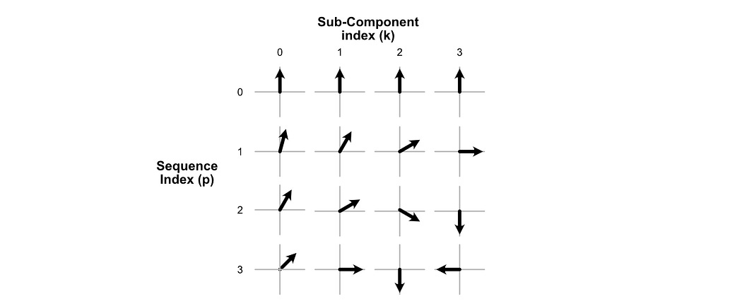
RoPE treats each of these vectors as a collection of small, 2D vectors. Then, RoPE rotates these sub-vectors depending on where they are in the input sequence.
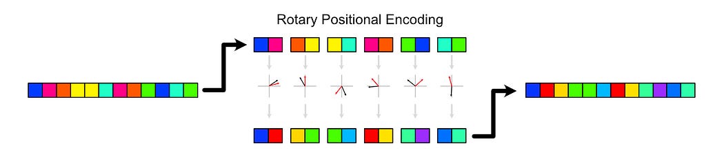
Naturally, if you rotate a vector all the way around, you end up with the same vector. If we want to encode long sequences with a lot of tokens, we need a way to encode a lot of positions without creating duplicates. We also, though, don’t want to make rotations so miniscule as to make it difficult for the model to understand the positional information we’re trying to encode.

RoPE deals with this by rotating different sub-vectors within each word vector by different amounts. Under the hood, actual rotation is done by multiplying a specially formed matrix by each individual sub-component.

This matrix has the parameter θ (theta), which specifies how much the vector is rotated. In RoPE, θ changes not only as a function of where a vector is within the sequence, but also which sub-component we’re operating on within each vector. Some sub-vectors are rotated quickly, while others are rotated slowly. This allows the model to be exposed to rotations that change quickly over time (communicating a lot of information, but repeating often) and slowly change over time (not communicating a lot of granular information, but also never repeating).

Here, θ is fed into the rotation matrix to govern how much a particular matrix is rotated. p represents the index of a word vector within a sequence. ωk represents the speed at which the kth vector rotates, which is defined by 10000^(-2k/d). Here. k is which sub-component of the vector we’re operating on, and d is the total length of the vector.
This has strong conceptual ties to the additive sinusoidal positional encoding strategy we discussed previously.

RoPE is relatively straightforward conceptually, but it (and derivative approaches like XPos and YaRN) contain subtle qualities which are worth discussing in their own article. I’ll likely be doing dedicated IAEE and By-Hand articles on the subject in the near future. For now, we can cap off our understanding by studying an implementation of the approach.
import torch
import torch.nn as nn
import math

# --- Config ---
device = "cuda" if torch.cuda.is_available() else "cpu"
vocab_size = 20
d_model = 16
n_heads = 4
train_seq_len = 64
num_train = 30000
num_test = 500
batch_size = 256
epochs = 10
num_layers = 2

# --- Data: Predict index of max token ---
def generate_batch(num, seq_len):
    x = torch.randint(1, vocab_size, (num, seq_len))
    y = torch.argmax(x, dim=1)
    return x.to(device), y.to(device)

# --- RoPE ---
def apply_rope(x):
    b, seq_len, d = x.shape
    assert d % 2 == 0
    half_d = d // 2
    x = x.view(b, seq_len, half_d, 2)

    freqs = torch.arange(half_d, device=x.device).float()
    theta = 10000 ** (-freqs / half_d)
    pos = torch.arange(seq_len, device=x.device).float()
    angles = torch.einsum("s,f->sf", pos, theta)

    cos = torch.cos(angles).unsqueeze(0).unsqueeze(-1)
    sin = torch.sin(angles).unsqueeze(0).unsqueeze(-1)

    x1 = x[..., 0:1] * cos - x[..., 1:2] * sin
    x2 = x[..., 0:1] * sin + x[..., 1:2] * cos

    x_rot = torch.cat([x1, x2], dim=-1)
    return x_rot.view(b, seq_len, d)

# --- RoPE-aware Multihead Attention ---
class RoPEAttention(nn.Module):
    def __init__(self, d_model, n_heads):
        super().__init__()
        self.attn = nn.MultiheadAttention(d_model, n_heads, batch_first=True)
        self.norm = nn.LayerNorm(d_model)

    def forward(self, x):
        residual = x
        x = apply_rope(x)
        x, _ = self.attn(x, x, x)
        return self.norm(x + residual)

# --- Transformer Encoder Layer ---
class RoPEEncoderLayer(nn.Module):
    def __init__(self, d_model, n_heads):
        super().__init__()
        self.self_attn = RoPEAttention(d_model, n_heads)
        self.ff = nn.Sequential(
            nn.Linear(d_model, d_model * 4),
            nn.ReLU(),
            nn.Linear(d_model * 4, d_model)
        )
        self.norm = nn.LayerNorm(d_model)

    def forward(self, x):
        x = self.self_attn(x)
        x = x + self.ff(self.norm(x))
        return x

# --- Transformer Model with RoPE ---
class MaxIndexTransformer(nn.Module):
    def __init__(self, seq_len, num_layers):
        super().__init__()
        self.token_emb = nn.Embedding(vocab_size, d_model)
        self.layers = nn.ModuleList([
            RoPEEncoderLayer(d_model, n_heads) for _ in range(num_layers)
        ])
        self.norm = nn.LayerNorm(d_model)
        self.classifier = nn.Linear(d_model, 1)

    def forward(self, x):
        tok = self.token_emb(x)
        for layer in self.layers:
            tok = layer(tok)
        tok = self.norm(tok)
        logits = self.classifier(tok).squeeze(-1)  # [B, T]
        return logits

# --- Train ---
def train(model, optimizer, criterion):
    model.train()
    for _ in range(epochs):
        for _ in range(num_train // batch_size):
            x, y = generate_batch(batch_size, train_seq_len)
            logits = model(x)
            loss = criterion(logits, y)
            optimizer.zero_grad()
            loss.backward()
            optimizer.step()

# --- Evaluate ---
@torch.no_grad()
def evaluate(model, seq_len):
    model.eval()
    x, y = generate_batch(num_test, seq_len)
    logits = model(x)
    preds = torch.argmax(logits, dim=1)
    acc = (preds == y).float().mean().item()
    print(f"Eval acc at seq_len={seq_len}: {acc:.3f}")
    return acc

# --- Run ---
model = MaxIndexTransformer(seq_len=train_seq_len, num_layers=num_layers).to(device)
optimizer = torch.optim.Adam(model.parameters(), lr=1e-3)
criterion = nn.CrossEntropyLoss()

train(model, optimizer, criterion)
evaluate(model, train_seq_len)
Here, we see a lot of the usual suspects. We’re applying a transformer style model (this time, one that utilizes RoPE for positional encoding), to our task of finding the index of the largest number in the sequence.
The main addition, here is the apply_rope function
# --- RoPE ---
def apply_rope(x):
    b, seq_len, d = x.shape
    assert d % 2 == 0
    half_d = d // 2
    x = x.view(b, seq_len, half_d, 2)

    freqs = torch.arange(half_d, device=x.device).float()
    theta = 10000 ** (-freqs / half_d)
    pos = torch.arange(seq_len, device=x.device).float()
    angles = torch.einsum("s,f->sf", pos, theta)

    cos = torch.cos(angles).unsqueeze(0).unsqueeze(-1)
    sin = torch.sin(angles).unsqueeze(0).unsqueeze(-1)

    x1 = x[..., 0:1] * cos - x[..., 1:2] * sin
    x2 = x[..., 0:1] * sin + x[..., 1:2] * cos

    x_rot = torch.cat([x1, x2], dim=-1)
    return x_rot.view(b, seq_len, d)
I don’t want to get lost in the sauce in this article, but a bit of googling and GPTing can get you far if you want a thorough understanding of what every single line is doing. In essence, this function:
calculates key parameters based on the input sequence
creates the rotation matrix for each position
applies those rotations
returns the result
After running this code, we can see that the approach performs well on our toy problem.

Conclusion
In this article we covered positional encoding. We first discussed why it’s necessary, and how the original transformer tackled the problem with additive sinusoidal positional encoding. We then discussed a variety of different positional encoding strategies; learned positional encoding, relative positional encoding, bucketed relative positional encoding, and RoPE.
There are countless other positional encoding schemes out there, but I think the most important thing is to understand the general approach, why it’s necessary, and a few ways it can be done. In future article’s we’ll be exploring strategies that build on top of RoPE, so stay tuned!