


Graph Convolution — By Hand
Hand Computing A Fundamental Graph ML Approach


Graph Convolutional Networks (GCNs) are the most fundamental approach to applying machine learning to graph data. I discuss GCNs in depth in my article on the subject:

I also covered graphs, generally, in another article:

In this article, we’ll be working through the math of GCNs to build a better understanding of how they function mathematically.

Step 1: Defining The Graph and GCN Layer
As I discussed in my article on GCNs, a graph is a collection of nodes and edges.

Each node might have some set of features associated with it. This is often referred to as the “hidden state”. GCNs iteratively modify this hidden state by passing information between neighboring nodes. Here, H1 is the starting hidden state.

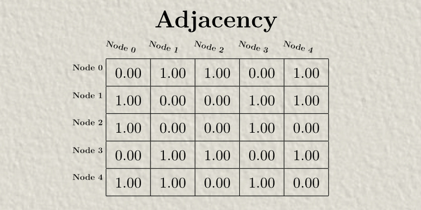
In GCNs, the way we keep track of connections between nodes is with an “Adjacency matrix”, which has a 1 where two nodes are connected and a 0 where two nodes are not connected.
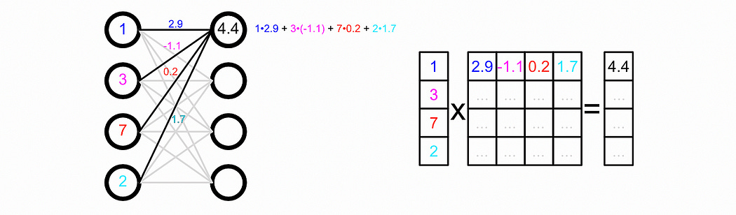
We’ll be using a 1-layer GCN in this example, which converts our hidden state H1 into a new hidden state H2 . We’ll be applying a Neural Network to all messages passed between nodes, which we call W1 . W1 represents a neural network.

This makes sense because, under the hood “passing data through a neural network” is actually matrix multiplication.
Notice that the W1 matrix is 3 x 2 in shape. This will convert the three features in the H1 matrix into two features in the H2 matrix. By manipulating the shape of the weight matrix, you can change how many features a particular GCN layer will output.
We’ll only be employing a one-layer GCN in this example, but multiple layers could be used, each of which would have their own weight matrix.
Step 2: Modifying The A Matrix and constructing the D Matrix
We’ll be using the edges between nodes to pass messages in our GCN. Recall the adjacency matrix, which specifies the edges of the graph.
Notice how there is no edge connecting Node0 to Node0. The only edges (where adjacency = 1) are between two different nodes.
This is common when defining a graph. However, in this application, we’ll be passing messages between nodes to update those nodes, and we’ll be doing that by passing along edges. If we want a node's previous hidden state to influence the next hidden state, all of the nodes need to have edges to themselves. We do this by specifying 1s along the diagonal.

One important idea in graph convolution is that the strength of a message coming from a particular node is scaled down by the number of connections that node has. This is an important step that allows less connected nodes to still have an impact while very connected nodes don’t wash out information from other nodes.
To do this, we construct a degree matrix, which specifies the number of connections each node has.

We then use this degree matrix to scale down the influence of highly connected nodes in a process called “normalization”.
Step 3: Normalizing
In normalization in GCNs, we scale down the strength of the messages being sent by the number of connections each node has. This means that a particular node with many connections won’t dominate the graph. If we were dealing with numbers then normalization would be easy, we would simply divide messages by the number of connections a node has. However, we are dealing with matrices, and matrices have no concept of division, so we can’t easily “divide” things. To get around this problem, we’ll use matrix inverses.
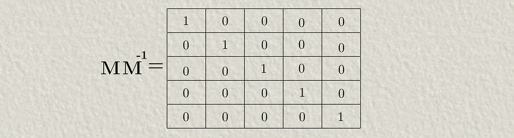
Calculating an inverse of a matrix is roundabout and unintuitive, but the idea is that a matrix times the inverse of that matrix is an identity matrix (an identity matrix having ones along the diagonal). This is conceptually similar to the idea that a number times the inverse of that number is equal to 1.
The actual process for calculating the inverse of a matrix can be complicated and has to do with “eigenvectors”, which I don’t want to get into in this article. Luckily, the degree matrix is a diagonal matrix (meaning there are only values on the diagonal), so calculating the inverse of the degree matrix is as easy as calculating the inverse of all the elements.

In theory, if we multiplied the adjacency matrix by the inverse of the degree matrix, we would scale down the adjacencies based on how well-connected nodes are. However, if you refer to the graph convolution equation, we don’t do that.
We actually multiply the adjacency matrix by the inverse square root of the degree matrix, both before and after. The reason we do that is because matrix multiplication is non-symmetrical; you multiply the rows of the first matrix by the columns of the second matrix. Thus, if you tried to normalize by multiplying by the inverse of the degree matrix, you would be preferentially normalizing certain nodes asymmetrically. We multiply by the inverse square root to, in essence, do half of our normalization row-wise, and half of our normalization column-wise.
So, first, we need to calculate the inverse square root. Because we’re dealing with a diagonal matrix we raise all of the values to ^(-1/2).

Then we can multiply that by the adjacency matrix to do half of the normalization process.

Then we can multiply by the other half to fully normalize our adjacency matrix.

Now the adjacency matrix is normalized by our degree matrix, meaning edges connecting nodes with a lot of edges are scaled down, and nodes with few edges are scaled up.
Step 4: Message Passing
The reason we normalized our adjacency matrix was to do message passing. Basically, we’ll use our adjacency matrix to make the hidden state of a node equal to an aggregate of messages passed from all other nodes. We do that by multiplying our normalized adjacency matrix by our hidden state matrix.

What makes this a machine learning model is that we then multiply the results of message passing by a weight matrix. Thus, the result of mixing hidden states based on the connections in the graph is passed through a neural network.
Here, the weight matrix is 3x2, which means we’re turning the three previous features for each node into two features. In the result, each row represents a node and each column represents a feature.

Then, like most neural networks, we pass that through a non-linear activation function like ReLU. This defines the hidden state for the next layer of graph convolution.

Thus, we’ve implemented a single layer of graph convolution. Multiple layers can be created, each with their own corresponding weight matrix, to do multiple layers of message passing; allowing graph convolutional networks to form subtle and complex interpretations of graph data.
Conclusion
And that’s it. In this article, we covered the major steps to computing graph convolution:
Defined a graph in terms of GCNs
Constructed the modified adjacency and degree matrix
Normalized the adjacency matrix by the degree matrix, to minimize the impact of nodes with too many connections
Performed message passing and passed the messages through a neural network, resulting in the new hidden state of the graph
Great stuff!