Self-Supervised Learning Using Projection Heads
Boost performance with unlabeled data
In this post you’ll learn about self-supervised learning, how it can be used to boost model performance, and the role projection heads play in the self-supervised learning process. We will cover the intuition, some literature, and a computer vision example in PyTorch.
Who is this useful for? Anyone who has unlabeled and augmentable data.
How advanced is this post? The beginning of this post is conceptually accessible to beginners, but the example is more focused on intermediate and advanced data scientists.
Pre-requisites: A high level understanding of convolutional and dense networks.
Code: Full code can be found here.
Self-Supervision vs Other Approaches
Generally, when one thinks of models, they consider two camps: supervised and unsupervised models.
Supervised Learning is the process of training a model based on labeled information. When training a model to predict if images contain cats or dogs, for instance, one curates a set of images which are labeled as having a cat or a dog, then trains the model (using gradient descent) to understand the difference between images with cats and dogs.
Unsupervised Learning is the process of giving some sort of model unlabeled information, and extracting useful inferences through some sort of transformation of the data. A classic example of unsupervised learning is clustering; where groups of information are extracted from un-grouped data based on local position.
Self-supervised learning is somewhere in between. Self-supervision uses labels that are generated programmatically, not by humans. In some ways it’s supervised because the model learns from labeled data, but in other ways it’s unsupervised because no labels are provided to the training algorithm. Hence self-supervised.
Self-supervised learning (SSL) aims to produce useful feature representations without access to any human-labeled data annotations. — K Gupta Et al.
Self-Supervision in a Nutshell
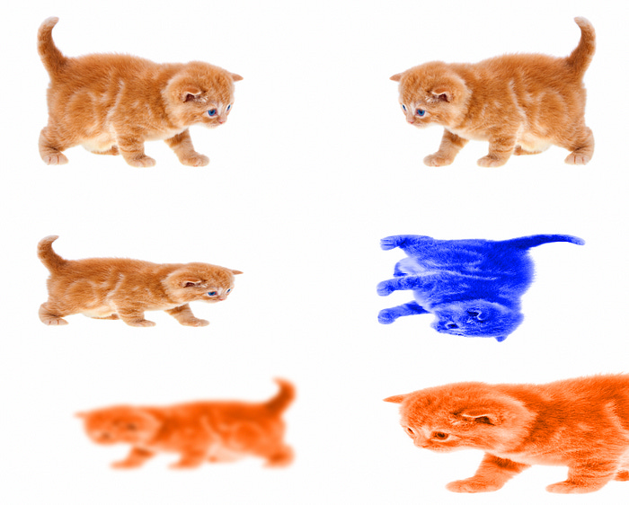
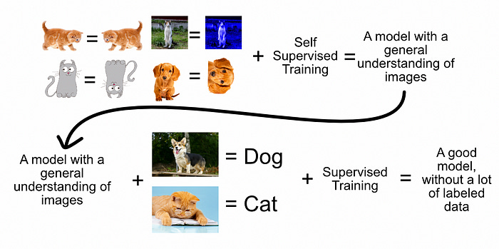
Self supervision uses transformations to the data, along with a clever loss function, to teach the model to understand similar data. We might not know what an image contains (it’s unlabeled by a human), but we do know a slightly modified image of a something is still an image of a that thing. As a result, you can label an image, and a flipped picture of an image, as containing the same thing.

The idea is, by training a model to learn if the data contains similar things, you are teaching the model to understand data regardless of how it is presented. In other words, You are training the model to understand the images, generally, regardless of class. Once self-supervision is done, the model can be refined on a small amount of labeled data to understand the final task (is an image of a dog or a cat).
I’m using images in this example, but self-supervision can be applied to any data that has augmentations that alter the data without modifying their essence from the perspective of the final modeling problem. For example, augmentation of audio data can be done using wave tables, which I describe in this article.
p.s. Another common way to conceptualize this is style invariance. In other words, you’re training a model to be good at ignoring stylistic differences in images.
Projection Heads
As machine learning has progressed as a discipline, certain architectural choices have proven to be generally useful. In convolutional networks, for instance, some networks have backbones, some have necks, and some have heads. The head, generally, is a dense network at the end of a larger network which turns features into a final output.

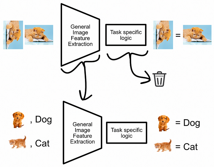
the function of this head is often described as a projection. Throughout math and many other disciplines, a projection is the idea of mapping something in one space to another space, like how a light from a lamp can map your 3d form into a 2d shadow on the wall. A projection head is a dense network at the end of a larger network tasked with transforming some information to other information. In our toy example of cats vs dogs, the projection head would project the general understanding of images as features into a prediction of cat vs dog.
Why Projection Heads are So Important in Self-Supervision.
Imagine you’re playing monopoly. There’s a lot to learn; investing in real-estate can pay dividends, it’s important to consider the future before making investments, pass go and collect $200, there’s no fundamental difference between a shoe and a thimble, etc. Within the game of monopoly there are two types of information: generally applicable and task specific information. You should not get excited every time you see the word “go” in your daily life: that’s task specific. You should, however, consider your investments carefully: that’s generally useful.
We can think of self supervision as a “game”, where the model learns to recognize similar or dissimilar images. Through playing this game, it learns to generally understand images, as well as specific rules in realizing if two images are the same image.

Once we have trained a self supervised model on similar data, and we now want to refine this model based on labeled data, we don’t care about the task specific logic to identify if two images are the same. We want to keep the general image understanding, but replace the task specific knowledge with classification knowledge. To do this, we throw out the projection head, and replace it with a new one.

The use of projection heads during the self-supervised learning process is a current point of research (this is a good paper on the subject), but the intuition is this: in self supervised learning You have to have the necessary logic to get good at the self supervised task so that you can learn generally applicable feature representations. Once you learn those features, the projection head, which contains the logic specific to optimizing self supervision, can be discarded.
Creating and using a projection head is a bit different than traditional modeling. The objective of the projection head isn’t necessarily to make a model which is good at the self-supervised task, but entice the creation of feature representations which are more useful in later, downstream tasks.
Self-Supervision in PyTorch
In this example we will be using a modification of the MNIST dataset, which is a classic dataset consisting of images of written numbers, paired with labels denoting which number the image represents.
MNIST consists of 60,000 labeled training images, and 10,000 labeled test images. In this example, however, We will discard all but 200 of the training labels. That means we will have a set of 200 labeled images to train from, and 59,800 unlabeled images to train from. This modification reflects the types of applications in which self supervision is most useful: Datasets with a lot of data, but which are expensive to label.
Full code can be found here.
The MNIST dataset is licensed under GNU General Public License v3.0, and the torchvision module used to load it is licensed under BSD 3-Clause “New” or “Revised” License, both permitting commercial use.
1) Load the Data
Loading the dataset
"""
Downloading and rendering sample MNIST data
"""

#torch setup
import torch
import torchvision
import torchvision.datasets as datasets
device = 'cuda' if torch.cuda.is_available() else 'cpu'

#downloading mnist
mnist_trainset = datasets.MNIST(root='./data', train=True,
                                download=True, transform=None)
mnist_testset = datasets.MNIST(root='./data', train=False,
                               download=True, transform=None)

#printing lengths
print('length of the training set: {}'.format(len(mnist_trainset)))
print('length of the test set: {}'.format(len(mnist_testset)))

#rendering a few examples
for i in range(3):
  print('the number {}:'.format(mnist_trainset[i][1]))
mnist_trainset[i][0].show()2) Separate into labeled and unlabeled data
In this example we will artificially ignore most of the labels in the training set to mimic a use case where it is easy to collect large amounts of data, but difficult or resource intensive to label all of the data. This code block also does some of the necessary data manipulation necessary to leverage PyTorch.
"""
Creating un-labled data, and handling necessary data preprocessing
"""

from tqdm import tqdm
import numpy as np
from sklearn.preprocessing import OneHotEncoder

# ========== Data Extraction ==========
# unlabeling some data, and one hot encoding the labels which remain
# =====================================

partition_index = 200

def one_hot(y):
  #For converting a numpy array of 0-9 into a one hot encoding of vectors of length 10
  b = np.zeros((y.size, y.max() + 1))
  b[np.arange(y.size), y] = 1
  return b

print('processing labeld training x and y')
train_x = np.asarray([np.asarray(mnist_trainset[i][0]) for i in tqdm(range(partition_index))])
train_y = one_hot(np.asarray([np.asarray(mnist_trainset[i][1]) for i in tqdm(range(partition_index))]))

print('processing unlabled training data')
train_unlabled = np.asarray([np.asarray(mnist_trainset[i][0]) for i in tqdm(range(partition_index,len(mnist_trainset)))])

print('processing labeld test x and y')
test_x = np.asarray([np.asarray(mnist_testset[i][0]) for i in tqdm(range(len(mnist_testset)))])
test_y = one_hot(np.asarray([np.asarray(mnist_testset[i][1]) for i in tqdm(range(len(mnist_testset)))]))

# ========== Data Reformatting ==========
# adding a channel dimension and converting to pytorch
# =====================================

#adding a dimension to all X values to put them in the proper shape
#(batch size, channels, x, y)
print('reformatting shape...')
train_x = np.expand_dims(train_x, 1)
train_unlabled = np.expand_dims(train_unlabled, 1)
test_x = np.expand_dims(test_x, 1)

#converting data to pytorch type
torch_train_x = torch.tensor(train_x.astype(np.float32), requires_grad=True).to(device)
torch_train_y = torch.tensor(train_y).to(device)
torch_test_x = torch.tensor(test_x.astype(np.float32), requires_grad=True).to(device)
torch_test_y = torch.tensor(test_y).to(device)
torch_train_unlabled = torch.tensor(train_unlabled.astype(np.float32), requires_grad=True).to(device)

print('done')3) Defining Model
To speed up training, this problem uses a super simple conv net and minimal hyperparameter exploration. This model has two general parts: the convolutional backbone and the densely connected head.
"""
Using PyTorch to create a modified, smaller version of AlexNet
"""
import torch.nn.functional as F
import torch.nn as nn

#defining model backbone
class Backbone(nn.Module):
    def __init__(self):
        super(Backbone, self).__init__()
        self.conv1 = nn.Conv2d(1, 16, 3)
        self.conv2 = nn.Conv2d(16, 16, 3)
        self.conv3 = nn.Conv2d(16, 32, 3)

        if torch.cuda.is_available():
            self.cuda()

    def forward(self, x):
        x = F.max_pool2d(F.relu(self.conv1(x)), 2)
        x = F.max_pool2d(F.relu(self.conv2(x)), 2)
        x = F.max_pool2d(F.relu(self.conv3(x)), 2)
        x = torch.flatten(x, 1)
        return x

#defining model head
class Head(nn.Module):
    def __init__(self, n_class=10):
        super(Head, self).__init__()
        self.fc1 = nn.Linear(32, 32)
        self.fc2 = nn.Linear(32, 16)
        self.fc3 = nn.Linear(16, n_class)

        if torch.cuda.is_available():
            self.cuda()

    def forward(self, x):
        x = F.relu(self.fc1(x))
        x = F.relu(self.fc2(x))
        x = self.fc3(x)
        return F.softmax(x,1)


#defining full model
class Model(nn.Module):
    def __init__(self):
        super(Model, self).__init__()
        self.backbone = Backbone()
        self.head = Head()

        if torch.cuda.is_available():
            self.cuda()

    def forward(self, x):
        x = self.backbone(x)
        x = self.head(x)
        return x

model_baseline = Model()
print(model_baseline(torch_train_x[:1]).shape)
model_baseline4) Train and test using only supervised learning as a baseline
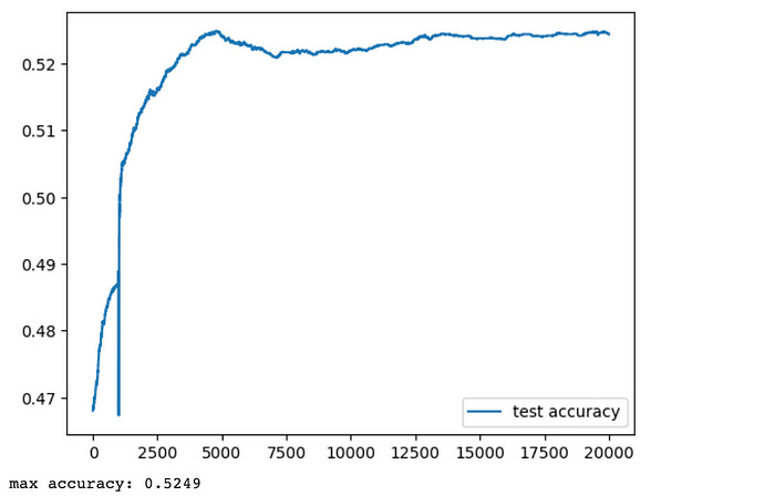
To get an idea of how much self supervision improves performance, we’ll train our baseline model on only the 200 labeled samples.
"""
Training model using only supervised learning, and rendering the results.
This supervised training function is reused in the future for fine tuning
"""

def supervised_train(model):

    #defining key hyperparamaters explicitly (instead of hyperparamater search)
    batch_size = 64
    lr = 0.001
    momentum = 0.9
    num_epochs = 20000

    #defining a stocastic gradient descent optimizer
    optimizer = torch.optim.SGD(model.parameters(), lr=lr, momentum=momentum)

    #defining loss function
    loss_fn = torch.nn.CrossEntropyLoss()

    train_hist = []
    test_hist = []
    test_accuracy = []

    for epoch in tqdm(range(num_epochs)):

        #iterating over all batches
        for i in range(int(len(train_x)/batch_size)-1):

            #Put the model in training mode, so that things like dropout work
            model.train(True)

            # Zero gradients
            optimizer.zero_grad()

            #extracting X and y values from the batch
            X = torch_train_x[i*batch_size: (i+1)*batch_size]
            y = torch_train_y[i*batch_size: (i+1)*batch_size]

            # Make predictions for this batch
            y_pred = model(X)

            #compute gradients
            loss_fn(model(X), y).backward()

            # Adjust learning weights
            optimizer.step()

        with torch.no_grad():

            #Disable things like dropout, if they exist
            model.train(False)

            #calculating epoch training and test loss
            train_loss = loss_fn(model(torch_train_x), torch_train_y).cpu().numpy()
            y_pred_test = model(torch_test_x)
            test_loss = loss_fn(y_pred_test, torch_test_y).cpu().numpy()

            train_hist.append(train_loss)
            test_hist.append(test_loss)

            #computing test accuracy
            matches = np.equal(np.argmax(y_pred_test.cpu().numpy(), axis=1), np.argmax(torch_test_y.cpu().numpy(), axis=1))
            test_accuracy.append(matches.sum()/len(matches))

    import matplotlib.pyplot as plt
    plt.plot(train_hist, label = 'train loss')
    plt.plot(test_hist, label = 'test loss')
    plt.legend()
    plt.show()
    plt.plot(test_accuracy, label = 'test accuracy')
    plt.legend()
    plt.show()

    maxacc = max(test_accuracy)
    print('max accuracy: {}'.format(maxacc))

    return maxacc

supervised_maxacc = supervised_train(model_baseline)
5) Defining Augmentations
Self supervised learning requires augmentations. This function augments a batch of images twice, resulting in a pair of stochastically augmented images to be used in contrastive learning.
import torch
import torchvision.transforms as T

class Augment:
   """
   A stochastic data augmentation module
   Transforms any given data example randomly
   resulting in two correlated views of the same example,
   denoted x ̃i and x ̃j, which we consider as a positive pair.
   """

   def __init__(self):

       blur = T.GaussianBlur((3, 3), (0.1, 2.0))

       self.train_transform = torch.nn.Sequential(
           T.RandomAffine(degrees = (-50,50), translate = (0.1,0.1), scale=(0.5,1.5), shear=0.2),
           T.RandomPerspective(0.4,0.5),
           T.RandomPerspective(0.2,0.5),
           T.RandomPerspective(0.2,0.5),
           T.RandomApply([blur], p=0.25),
           T.RandomApply([blur], p=0.25)
       )

   def __call__(self, x):
       return self.train_transform(x), self.train_transform(x)

"""
Generating Test Augmentation
"""
a = Augment()
aug = a(torch_train_unlabled[0:100])

i=1
f, axarr = plt.subplots(2,2)
#positive pair
axarr[0,0].imshow(aug[0].cpu().detach().numpy()[i,0])
axarr[0,1].imshow(aug[1].cpu().detach().numpy()[i,0])
#another positive pair
axarr[1,0].imshow(aug[0].cpu().detach().numpy()[i+1,0])
axarr[1,1].imshow(aug[1].cpu().detach().numpy()[i+1,0])
plt.show()6) Defining Contrastive Loss
Contrastive loss is the loss function used to entice positive pairs to be positioned closely in an embedding space, and negative pairs to be positioned further apart.
class ContrastiveLoss(nn.Module):
   """
   Vanilla Contrastive loss, also called InfoNceLoss as in SimCLR paper
   """
   def __init__(self, batch_size, temperature=0.5):
       """
       Defining certain constants used between calculations. The mask is important
       in understanding which are positive and negative examples. For more
       information see https://theaisummer.com/simclr/
       """
       super().__init__()
       self.batch_size = batch_size
       self.temperature = temperature
       self.mask = (~torch.eye(batch_size * 2, batch_size * 2, dtype=bool)).float().to(device)

   def calc_similarity_batch(self, a, b):
       """
       Defines the cosin similarity between one example, and all other examples.
       For more information see https://theaisummer.com/simclr/
       """
       representations = torch.cat([a, b], dim=0)
       return F.cosine_similarity(representations.unsqueeze(1), representations.unsqueeze(0), dim=2)

   def forward(self, proj_1, proj_2):
       """
       The actual loss function, where proj_1 and proj_2 are embeddings from the
       projection head. This function calculates the cosin similarity between
       all vectors, and rewards closeness between examples which come from the
       same example, and farness for examples which do not. For more information
       see https://theaisummer.com/simclr/
       """
       batch_size = proj_1.shape[0]
       z_i = F.normalize(proj_1, p=2, dim=1)
       z_j = F.normalize(proj_2, p=2, dim=1)

       similarity_matrix = self.calc_similarity_batch(z_i, z_j)

       sim_ij = torch.diag(similarity_matrix, batch_size)
       sim_ji = torch.diag(similarity_matrix, -batch_size)

       positives = torch.cat([sim_ij, sim_ji], dim=0)

       nominator = torch.exp(positives / self.temperature)

       denominator = self.mask * torch.exp(similarity_matrix / self.temperature)

       all_losses = -torch.log(nominator / torch.sum(denominator, dim=1))
       loss = torch.sum(all_losses) / (2 * self.batch_size)
       return loss

"""
testing
"""
loss = ContrastiveLoss(torch_train_x.shape[0]).forward
fake_proj_0, fake_proj_1 = a(torch_train_x)
fake_proj_0 = fake_proj_0[:,0,:,0]
fake_proj_1 = fake_proj_1[:,0,:,0]
loss(fake_proj_0, fake_proj_1)
7) Self Supervised Training
Training the model to understand image similarity and difference via self supervision and contrastive loss. Because this is an intermediary step, it’s difficult to create clear and intuitive performance indicators. As a result, I opted to spend some extra compute to intimately understand loss, which was useful in tuning parameters to get consistent model improvement.


