
Transformer XL Positional Encoding —By Hand
A by-hand breakdown of relative positional encoding with content-dependent and global bias terms


I recently released a piece that explores various positional encoding strategies in-depth. This article is meant to be a companion piece to that article, and explores relative positional encoding with content-dependent and global bias terms from the Transformer XL paper. This is an early relative positional encoding scheme designed to allow LLMs to better and more efficiently understand arbitrarily long sequences.
Like other installments in the By-Hand series, this article is designed to serve as a brief reference rather than an exhaustive breakdown. For a conceptual breakdown, see the following IAEE article:

This article assumes a strong working knowledge of attention in general. I have beginner friendly IAEE articles on the subject

As well as By-Hand articles on classic attention approaches.


Step 1: Defining the Inputs and Parameters
First, we need to convert our input sequence to a vector embedding, usually by using a lookup of vectors that are optimized through the training process.
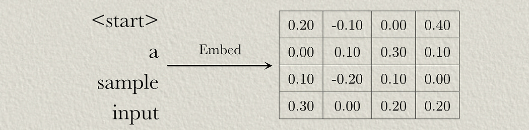
So, in this example, we have a sequence length of 4 and a modeling dimension of 4 (the length of the vector used to encode each word).
The positional encoding scheme we’re discussing uses four weight matrices and two bias vectors. These would be randomly initialized then updated throughout the training process.
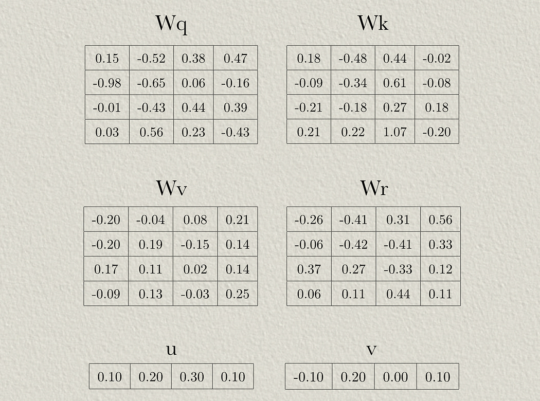
These parameters represent the following:
Wq is the weights used to project the input into the query of self attention (just like in traditional attention mechanisms).
Wk is the weights used to project the input into the key of self attention (just like in traditional attention mechanisms).
Wv is the weights used to project the input into the value of self attention (just like in traditional attention mechanisms).
Wr are weights used to apply locational information to the attention mechanism
u allows the attention mechanism to learn biases to content information
v allows the model to learn biases to positional information
We’ll explore exactly how these works in the following sections.
In this article, we’ll imagine a simple model consisting of a single attention block. Naturally, a real model would have many decoder blocks with many layers of attention. In such a model, each attention block would have its own parameters. This means each attention layer learns positional information independently.
Step 2: Calculating Relative Positional Encoding
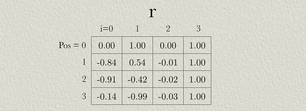
Transformer XL uses sinusoidal positional encoding, similar to the original transformer. The following function can be used to calculate the positional encoding at a particular index:

here:
pos is the position in the sequence a particular word is (word 1, word 2, word 3, etc).
i is the position in each word embedding a value is in (value 1 in word 1, value 2 in word 1, value 3 in word 1, etc).
d the modeling dimension (the length of the vectors in the model, in this case 4).
One major difference between the original transformer and transformer XL is what pos represents. In the original transformer pos represents the location in the sequence
0, 1, 2, 3, 4, 5, 6, .... nWhereas, in Transformer XL, pos represents the distance relative to the current last token
n ... , 6, 5, 4, 3, 2, 1, 0This means that, no matter how long the sequence is, the positional encoding for the token three steps before the most recent token will always be the same. Because the text closest to the current token has the largest bearing on generation, this allows Transformer XL to generalize much more easily to longer sequences compared to absolute positional encoding.
For our sample input, we can calculate a positional encoding for each token, relative to the final token. here, pos=0 is the position of the final token, where pos=1 , pos=2 , etc. are preceding tokens.
Step 3: Projection
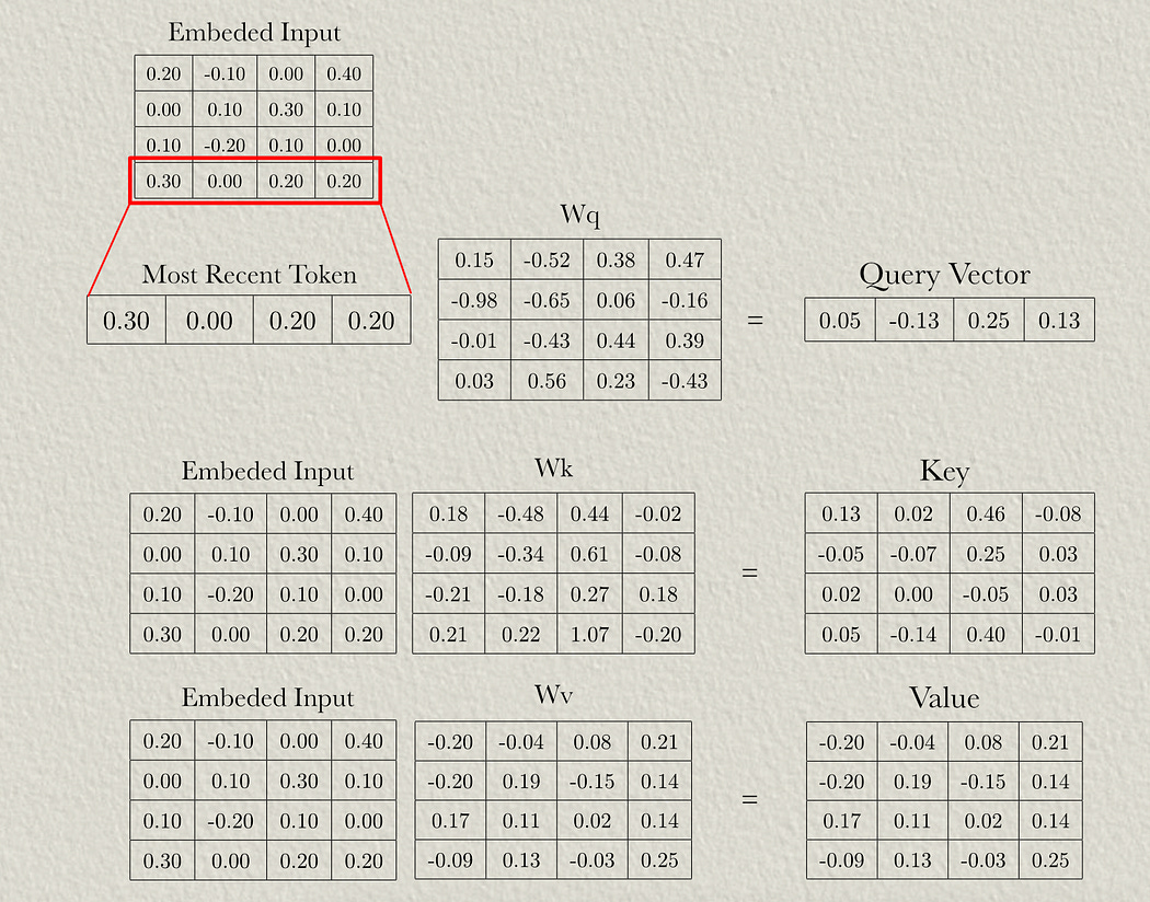
Just like any other flavor of attention, vectors representing words are passed through neural networks (represented as weight matricies), and those representations are used in attention calculations. The only real difference is that the location information is projected independently to allow the model to learn how to reason about location.
First, we can take the input embeddings and pass them through the a weight matrix to result in the query, key, and value like normal.
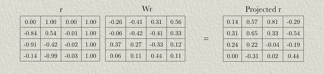
Then we can pass the relative positional matrix through its own weight matrix.
The model will use these projected values to construct a few different attention representations simultaneously.
Step 4: Calculating Terms and Attention Scores
Unlike earlier approaches that add positional information to the initial input to the model, Transformer XL injects positional information through each attention layer. In each head of each attention mechanism of the model, four terms are calculated:
Term a: Attention based on content
Term b: Attention based on a combination of content and position
Term c: Attention based on a global content bias
Term d: Attention based on a global position bias
These are all added together to create attention scores which incorporate both information about tokens as well as where they’re located
Term A
Term A is, essentially, classic attention. The Query and Key are multiplied together to construct attention scores.

“Term A”, in this image, represents attention scores pre soft-maxing. We’ll be softmaxing to calculate the actual attention values after we calculate all terms and add them together.
Term B
We can multiply the query by our projected r values to calculate term B.

Recall that Projected r is our relative positional encoding information that’s been passed through a neural network, allowing the query vector to interact with a learned representation of positional information.
Normally I don’t harp on the naming convention of “query” and “key”, but in this application I find an understanding of the naming convention is useful. our “projected r” matrix in term B, and the “key” matrix in term A can both be conceptualized as a database of values. When we multiply the query vector by these matrices, the query extracts information from these matrices.
We have the same query vector, representing the most recent token, and we’re applying that to different “databases” (conceptually) to extract different information.
Term C
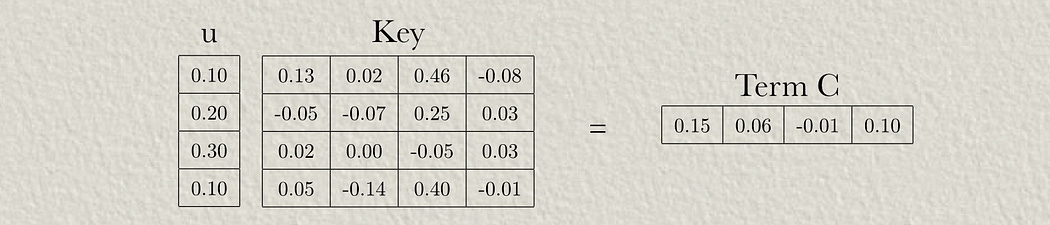
In the previous two terms we co-related the query vector with information about words. Terms C an d D allow the model to build its own vectors, u and v , to interact with information about words. The previous two terms are referred to as “content dependent”, because the query is derived from the input. Terms C and D are referred to as “global bias” terms because the parameters used in place of the query ( u and v ) are learned by the model and are not influenced by the input content.
Term C is the “global content bias”, meaning we multiply the learned vector u by the embedded word vectors.
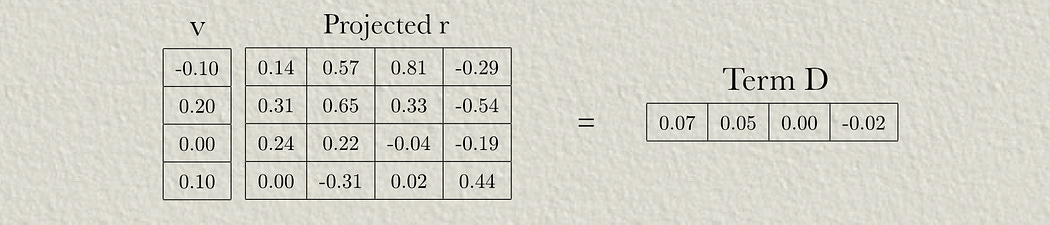
Term D
Term D is just like term C, accept a different learned vector ( v ) is applied to the learned positional information ( projected r ), instead of the content ( key ). Thus, term D represents the “global position bias”
Step 4: Calculating Attention and Applying to the Value Matrix
Now that we’ve calculated terms A, B, C, and D, we can add them together and softmax them to calculate aggregate attention scores.
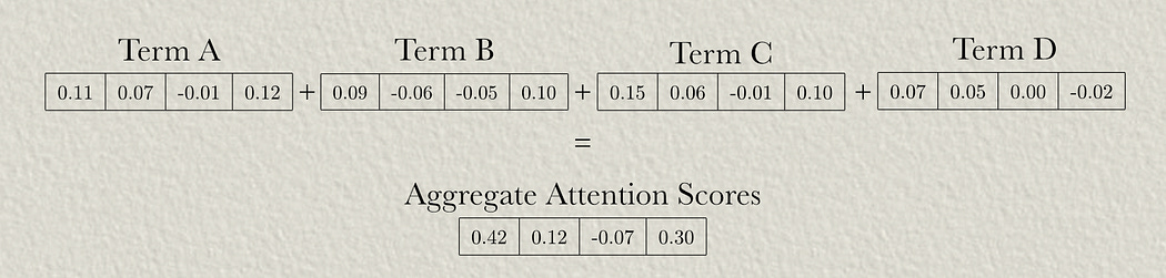
And then we can softmax them. Softmaxing is simple, but hard to draw (and I’m already way behind on publishing), so I’ll leave that as an exercise to the reader. Refer to my article on multi-headed self attention (step 7) for a reference on that.

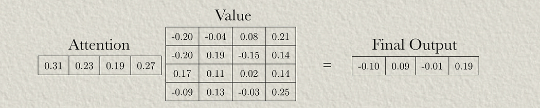
We can then apply those attention scores to the value matrix to calculate our result.
Discussion
The reason Transformer XL was created was to make decoder style model better at longer sequences. It did this in three key ways:
By making position relative to the token being generated. This allowed the model to generate to sequences longer than it was trained on
By making inferences of long sequences more efficient. One strategy to apply models to sequences which are longer than the context length they’re applied on is to treat them like a recurrent model. You essentially just trim off some of the sequence at the beginning so you have room at the end to generate data. If positional information is encoded in the vectors themselves, then you need to re-compute all of the attention layers for this entire process. With transformer XL, because locational information is calculated on the fly for each token generated, you can efficiently move the context window around.
If that’s all french, check out my article on positional encoding, which approaches this topic from a higher level.
Cheers!