YOLO is a landmark object detection model which can quickly classify and localize numerous objects within an image. This summary goes over all critical mathematical operations within a YOLO model. If you’d like to learn more about the intuition behind YOLO, check out the IAEE article.
Step 1: Defining the Input
To use a YOLO model, an RGB image must first be converted into a 448 x 448 x 3 tensor

We’ll be using a simplified 5 x 5 x 1 tensor so the math takes up less space.

Step 2: Layer Normalization
Neural networks typically perform better on normalized data. We can normalize the input by first computing the average value in the matrix (µ ).
Next, the absolute difference of all elements by the average can be calculated.

Then, the standard deviation can be calculated by squaring all values in the result of the previous section, adding them together, dividing by the number of values, and calculating the square root.

Once the standard deviation has been calculated, the input can be layer normalized by subtracting the mean and dividing by the standard deviation.
The mean is the average value of the input image, and the standard deviation is how broad the distribution of values is in original image. By subtracting by the mean and dividing by the standard deviation, we “normalize” the image.
Note: we calculated the layer norm. The original YOLO paper used batch norm, which normalizes the same values across different images in a batch. We calculated the layer norm. The conceptual difference between the two is negligible
Step 3: Convolution
Now that our input has been normalized, we’ll pass it through a convolutional network. We’ll idealize YOLO as a single convolutional layer with two kernels
To ensure the output tensor has the same spatial dimensions as the input, a pad of 0’s is applied to our normalized input
Then both kernels can be convolved over the image via element wise multiplication (⊙) and cumulative summation (Σ).
After both kernels have been convolved over the input, we get two arrays of equal size. These are typically represented as a 3D tensor where different kernels exist across a dimension called the “filter” or “kernel” dimension.
Step 4: Max Pooling
Now that we convolved our input, we can apply max pooling. In this example we max pool each convolved matrix with a 2 x 2 window of stride 2. We max pool partial sections as well. In this case I used an implementation of max pooling that sets the value to zero if all values are negative. Practically I think this has little impact.
Step 5: Non-Linear Activation
Virtually all ML models, YOLO included, employ non-linear “activation functions” throughout the model. As all math before this point has been linear (multiplication and addition) , the previous steps can only model linear relationships. Adding a function that maps values within the model non-linearly allows the model to learn non-linear relationships. In this example we’re using the sigmoid activation function, but ReLU is more common.
Note: it’s slightly more efficient to apply activation functions after max pooling.
This function can be applied to all max pooled matrices element wise

Step 6: Flattening
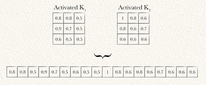
Now that the input image has been filtered into an abstract representation which is better suited for the end modeling task (in reality by several convolutions layers rather than the one convolutional layer in this example), it can be converted into a vector via flattening.
Step 7: Output Projection
A dense network (which is matrix multiplication) can be used to project the flattened matrix into the final output. The final output of YOLO consists of SxSxCclass predictions, and SxSxBx5bounding box predictions. Thus, the shape of the output must be of shape SxSx(C+Bx5). Assuming the output of flattening in the previous step has a length L, the weight matrix of the dense network must be of shape Lx(SxSx(C+Bx5)).
In this example we’ll assume S is 1, C is 2, and B is 1. L is the length of the flattened vector, which is 18. Therefore the shape of the weight matrix should be 18 x 7.
Note: matrices denoted with ` are visually transposed.
Class probabilities per square should add to 1. Thus, the predicted classes for each grid square are softmaxed.

Step 8: Inferencing
The final output of YOLO, in this example a 7 element long vector, has been calculated. Now we can use those values to generate our final inference. Because S = 1, there is only one grid cell. Because B = 1, there is only one bounding box. Because C = 2 there are two class predictions
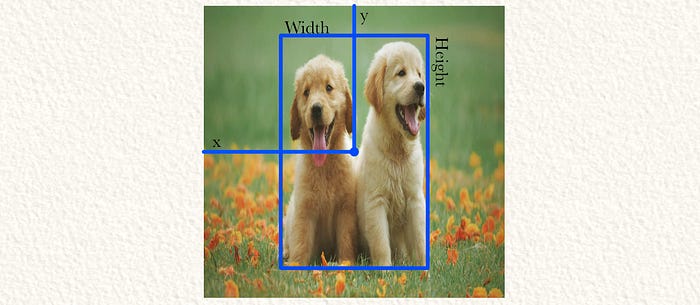
YOLO predicted that the grid cell (the entire image in this case) contains a dog. The bounding box is 50% off of the left wall and 50% off of the top wall of the cell. The width is 30% of the width of the cell, the height is 70% the height of the cell. Also, YOLO is 90% confident that this is a good bounding box.
In a less trivial example, where there are four grid cells (S=4) with one bounding box per cell:
The confidence for the top left and right cells is too low, so the bounding boxes aren’t used. The other two are used. Note that the height (and width) can be greater than 1, as the bounding box can be a multiple larger than the grid cell height.
Conclusion
And that’s it. In this article we covered the major steps to computing the output of YOLO:
Defining the input
Normalizing the input
Applying convolution
Applying max pooling
Non-linear activation
Flattening
Projection into the output shape
Composed our final inference
If you’re interested in understanding the theory, check out the IAEE article:
If you’ve enjoyed this article, subscribe for the highest quality Data Science content on the internet.
Feel free to share it with friends and colleagues. This article is free and publicly accessible to all readers.
Level up your AI skills be by joining the IAEE discord. Get access to weekly lectures and next level learning.


I would be thrilled to answer any questions or thoughts you might have about the article. An article is one thing, but an article combined with thoughts, ideas, and considerations holds much more educational power!