Convolutional Networks — Intuitively and Exhaustively Explained

Unpacking a cornerstone modeling strategy

“Convolved” by the author using MidJourney. All images by the author unless otherwise specified.

Convolutional neural networks are a mainstay in computer vision, signal processing, and a massive number of other machine learning tasks. They’re fairly straightforward and, as a result, many people take them for granted without really understanding them. In this article we’ll go over the theory of convolutional networks, intuitively and exhaustively, and we’ll explore their application within a few use cases.

Who is this useful for? Anyone interested in computer vision, signal analysis, or machine learning.

How advanced is this post? This is a very powerful, but very simple concept; great for beginners. This also might be a good refresher for seasoned data scientists, particularly in considering convolutions in various dimensions.

Pre-requisites: A general familiarity of with backpropagation and dense neural networks might be useful, but is not required. I cover both of those in this post:

What Are Gradients, and Why Do They Explode?

The Reason Convolutional Networks Exist

The first topic many fledgling data scientists explore is a dense neural network. This is the classic neural network consisting of nodes and edges which have certain learnable parameters. These parameters allow the model to learn subtle relationships about the topics they’re trained on.

A conceptual diagram of a dense network which takes in some inputs and predicts an output. It learns the necessary parameters to perform well at the task by incrementally learning from known examples (i.e. the success and failure of previous super bowl teams).

As the number of neurons grow within the network, the connections between layers become more and more abundant. This can allow complex reasoning, which is great, but the “denseness” of dense networks presents a problem when dealing with images.

Let’s say we wanted to train a dense neural network to predict if an image contains a dog or not. We might create a dense network which looks at each pixel of the image, then boil that information down to some final output.

A conceptual diagram of what hooking up an image to a dense network might look like

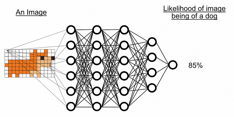
Already we’re experiencing a big problem. Skipping through some math to get to the point, for this tiny little network we would need 1,544 learnable parameters. For a larger image we would need a larger network. Say we have 64 neurons in the first layer and we want to learn to classify images that are 256x256 pixels. Just the first layer alone would be 8,388,608 parameters. That’s a lot of parameters for a, still, pretty tiny image.

Another problem with neural networks is their sensitivity to minor changes in an image. Say we made two representations of our dog image; one with the dog at the top of the image, and one with the dog at the bottom.

A neural network looking at the same pixel on two similar images

Even though these images are very similar to the human eye, their values from the perspective of a neural network are very different. The neural network not only has to logically define a dog, but also needs to make that logical definition of a dog robust to all sorts of changes in the image. This might be possible, but that means we need to feed the network a lot of training data, and because dense networks have such a large number of parameters, each of those training steps is going to take a long time to compute.

So, dense networks aren’t good at images; they’re too big and too sensitive to minor changes. In the next sections we’ll go over how convolutional networks address both of these issues, first by defining what a convolution is, then by describing how convolution is done within a neural network.

Convolution in a Nutshell

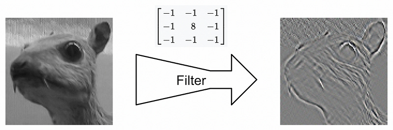
At the center of the Convolutional Network is the operation of “convolution”. A “convolution” is the act of “convolving” a “kernel” over some “target” in order to “filter” it. That’s a lot of words you may or may not be familiar with, so let’s break it down. We’ll use edge detection within an image as a sample use case.

A kernel, from a convolutional perspective, is a small array of numbers

An example of a kernel. This specific kernel is used in edge detection

This kernel can be used to transform an input image into another image. The act of using a standard operation to transform an input into an output is typically called “filtering” (think Instagram filters used to modify images).

The kernel gets used to filter an input image to an image which highlights edges in the original image. Generally the input image is sometimes referred to as the “target” image, while the output is sometimes referred to as the “filtered” image. Source

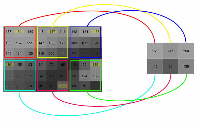
The filtering actually gets done with “convolution”. The kernel, which is much smaller than the input image, is placed in every possible position within the image. Then, at a given location, the values of the kernel are multiplied by values of the input image. The results are then summed together to define the value of the output image.

“convolving” the kernel across the target image. the 3x3 kernel gets applied to every 3x3 square of the target image. The values of the kernel are multiplied by the values of the pixels in the corresponding location, and then all values are added together. to construct a single pixel in the output image.

In machine learning convolutional is most often applied to images, but they work perfectly well in other domains. You can convolve a wavelet over a one dimensional signal, you can convolve a three dimensional tensor over a three dimensional space. Convolution can take place in an arbitrary number of dimensions.

An example of convolution in 1D, left, and convolution in 3D, right. both cases function similarly to 2D convolution; the kernel (depicted in blue) is swept over all possible locations (examples in red), the overlapping values are then multiplied and the results are summed together to construct a single output value.

We’ll stay in two dimensions for most of this article, but it’s important to keep the general aspect of convolutions in mind; they can be used for many problem types outside of computer vision.

So, now we know what convolution is and how it works. In the next section we’ll explore how this idea can be used to build models.

Convolutional Neural Networks in a Nutshell

The whole idea of a convolutional network is to use a combination of convolutions and downsampling to incrementally break down an image into a smaller and more meaningful representation. Typically this broken down representation of the image is then passed to a dense network to generate the final inference.

The high level architecture of a typical convolutional neural network. The actual convolutions typically exist within a “backbone” of convolutions and downsampling. Once the input has been condensed into a meaning-rich representation (also known as a bottleneck), the next step is typically a dense network, which is commonly referred to as a “head” or “projection head”, that generates the desired final response. I talk about these concepts a bit more in depth in another article about the importance of projection heads in self-supervised learning.

Similarly to a fully connected neural network which learns weights between connections to get better at a task, convolutional neural networks learn the values of kernels within the convolutional layers to get better at a task.

Recall how the kernel is swept through an image to transform it into a different representation. A convolutional network incrementally adjusts the values of the kernel to make a filtered image which is somehow better for the final modeling task.

There are many ways to downsample in a convolutional network, but the most common approach is max pooling. Max pooling is similar to convolution, in that a window is swept across an entire input. Unlike convolution, max pooling only preserves the maximum value from the window, not some combination of the entire window.

An example of max pooling applied to an image, which downsamples the image from 6x9 to 2x3. If you’re curious why these squares don’t overlap while convolution does, that’s because of “stride”, which we’ll cover in a later section.

So, through layers of a convolution and max pooling, an image is incrementally filtered and downsampled. Through each successive layer the image becomes more and more abstract, and smaller and smaller in size, until it contains an abstract and condensed representation of the image.

And that’s were a lot of people stop in terms of theory. However, convolutional neural networks have some more critical concepts which people often disregard. Particularly, the feature dimension and how convolution relates with it.

⚠️ Epilepsy Warning: The following sections contain rapidly moving animations⚠️

The Feature Dimension

You might have noticed, in some of the previous examples, we used grayscale images. In reality images typically have three color channels; red, green, and blue. In other words, an image has two spatial dimensions (width and height) and one feature dimension (color).

This idea of the feature dimension is critical to the thorough understanding of convolutional networks, so let’s look at a few examples:

Example 1) RGB images

Because an image contains two spatial dimension (height and width) and one feature dimension (color), an image can be conceptualized as three dimensional.

An image (on the left), the three channels that make up the image (middle), and the shape of the data which we’ll feed into the model (right)

Generally, convolutional networks move their kernel along all spatial dimensions, but not along the feature dimension. With a two dimensional input like an image one usually uses a 3D kernel, which has the same depth as the feature dimension, but a smaller width and height. This kernel is then swept through all spatial dimensions.

A conceptual animation of convolution of an image. a 3D kernel is applied to the entire feature dimension, and is swept through both spatial dimensions. This is a 2D convolution, because the actual traversal takes place in two dimensions. Note: the feature dimension is also commonly referred to as “channels”.

Typically, instead of doing one convolution, it’s advantageous to do multiple convolutions, each with different kernels. This allows the convolutional network to create multiple representations of the image. Each of these convolutions uses its own learnable kernel, and the representations are concatenated together along the feature axis.

A conceptual diagram of three kernels applied to the input image. Each of these kernels create their own feature layer. all the values in each of the kernels are learnable parameters.

As you may have inferred, you can have an arbitrary number of kernels, and can thus create a feature dimension of arbitrary depth. Many convolutional neural networks use a different number of features at various points within the model.

The architecture for the original YOLO model, a landmark convolutional model in image processing. Notice how the boxes in the diagram are three dimensional, these boxes represent the height, width, and number of features at various points throughout the model. Don’t worry too much about the text of this image just yet, we’ll revisit this diagram later. Source

Max pooling typically only considers a single feature layer at a time. In essence, we just do max pooling on each individual feature layer.

Conceptual diagram of maxpool applied to 3 features. Note, maxpool is typically applied after convolution, not before.

Those are the two main operations, convolution and max pooling, on a two dimensional RGB image.

Example 2) Stereo Audio

While time series signals like audio are typically thought of as one dimensional, they’re actually typically two dimensional, with one dimension representing time and another dimension representing multiple values at that time. For instance, stereo audio has two separate channels, one for the left ear and one for the right ear.

The left and right sound waves from a snippet of stereo trumpet music, in the time domain. The X axis corresponds to time, in seconds, and the y axis corresponds to the amplitude of the signal, which controls the location of a speaker diaphragm, generating sound. From my article on the frequency domain

This can be conceptualized as a signal with one spatial dimension (time) and one feature dimension (which ear).

Our stereo audio data can be conceptualized as two dimensional; a time dimension and a feature dimension.

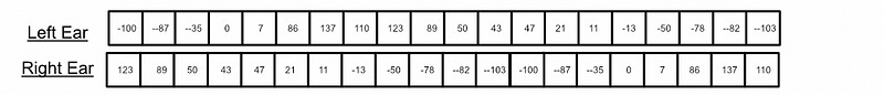
Applying convolutions and max pooling to this data is very similar to images, except instead of iterating over two dimensions, we only iterate over one.

A conceptual diagram of one dimensional convolution. In this example we have three simple kernels applied to the input. Recall that these kernels are learnable, and their values would change throughout model training.

Max pooling is also similar to the image approach discussed previously. We treat each row across the feature dimension separately, apply a moving window, and preserve the maximum within that window.

An example of max pooling. Each feature is divided into regions, and the maximum within those regions is preserved.

Example 3) MRI/CT scans

Depending on the application, data of scans can be conceptualized as three dimensional or two dimensional.

An animation of an MRI, slice by slice, of a human head. Typically this type of data is treated as a three dimensional problem. Image source

An example of a CT scan from the Vesuvius Ink Detection Challenge, a challenge involving reading carbonized scrolls from pompeii without needing to destroy them through unraveling. This data is of a two dimensional object with depth. Sometimes, this type of data is referred to as “2.5D” because there are two major spatial dimensions and a minor spatial dimension which can be conceptualized as a feature dimension. source

The example from the piece of paper can be treated as a 2D spatial data problem with a feature dimension representing depth. It’s really three dimensional, the paper has some thickness which is recorded by the CT scan, but the depth dimension is minor enough that it can be treated as a feature dimension. This would be just like our image example, except instead of a layer for every color, we would have a layer for every physical layer of data.

For the fully three dimensional scan of a human head, where it may not be useful to think of it as a flat object but as a full three dimensional object, we can use three dimensional convolution and max pooling. This is conceptually identical to the previous methods, but much harder to draw. We would do convolve over all three spatial dimensions, and depending on the number of kernels we employ, we would get a four dimensional output.

An example of employing two convolutional kernels across a given three dimensional dataset with a single feature. This results in two 3D outputs, one for each kernel. The output would thus be four dimensional.

Technically there’s no limit to the dimensionality of convolutional networks. You could do convolution in five, six, or one thousand dimensions. I think three was already hard enough, and the vast majority of convolutional models work on two dimensional data anyway, so we’ll end our example exploration here.

By this point you may have some fundamental questions like “do kernels always have to be a certain size”, or “do kernels always have to overlap?” We’ll cover questions like that in the next question.

Kernel Size, Stride, and Padding

While we previously considered all kernels to be of size three, there’s no limit to the size of a convolutional kernel. This configurable size is often referred to as the kernel size.

Kernels of size two, three, and four on a two dimensional task

I’ve also idealized all convolutions as only stepping one point at a time, but convolutions can step larger amounts, which is referred to as stride. Max pooling also has a stride parameter, which is often the size of the max pooling window. This is why I depicted max pooling as not overlapping.

Conceptual diagram of strides of length one (left), two (middle), and three (right), all for a kernel of size two.

Sometimes it’s advantageous to have the output size of a convolution equal to the input size of a convolution, but because kernels are typically larger than size one, any result of a convolution will necessarily be smaller than the input. As a result we can “pad” the borders of an image with some default value, maybe even a reflection of the input, in order to get an output that’s similarly sized. This general process is called padding.

Non Linear Activation Functions

Part of the thing that makes neural networks, in general, learn complex tasks is non-linearity. If we don’t use activation functions then, at the end of the day, convolutions can only create linear relationships (combinations of addition and multiplication). If we throw some activation functions in the mix, which map some input into an output non-linearly, we can get our convolutional network to learn much more complex relationships. The most common activation function used in convolutional networks is ReLu.

Typically, activation functions are applied after convolution and before max pooling, so something like this:

output = maxPool(relu(conv2d(input))

However, while it’s not a big difference, it is slightly more performant to swap maxPool and activation, which doesn’t end up impacting the final output.

output = relu(maxPool(conv2d(input))

regardless of how it’s done, adding non-linear activation functions within a model greatly increases the models ability to learn complex tasks.

Flattening and Dense Nets

Convolutional networks are good at breaking data down into it’s essence, but dense networks are better at doing logical inference. After passing data through a convolutional network, the data is often “flattened” then passed through a dense network.

Conceptual diagram of how flattenting relates to the greater convolutional modeling paradigm. Fully connected networks typically expect a list of data, and convolutional models typically come in higher than one dimension. The output of the conv. net is usually unraveled into a list before passing it to a dense network, an operation called flattening.

I have more information on the role of dense networks as “projection heads” in the following article:

Conclusion

And that’s it! I wouldn’t say we went over every possible approach or theory of convolutional networks (that would be a pretty long article), but we covered the theory necessary to understand pretty much every approach that exists. You should have an idea of why conv nets are better than dense nets for some applications, what a kernel is, what convolution is, and what max pooling is. You should have an understanding of the feature dimension and how it’s used across various 1D, 2D, and 3D use cases. You should also understand key parameters, like kernel size, padding, and stride.

Take a look at the YOLO diagram, and consider how kernel size, stride, number of features/kernels, flattening, and dense networks relate to the diagram. Source

---

Attribution: All of the resources in this document were created by Daniel Warfield, unless a source is otherwise provided. You can use any resource in this post for your own non-commercial purposes, so long as you reference this article, https://danielwarfield.dev, or both. An explicit commercial license may be granted upon request.